Functions 8: SUMIF, COUNTIF & AVERAGEIF
Time to learn: 30 minutes
Need a detailed report fast? Need to get the breakdown of sums, averages or a count of your data? Need to get them by SEPARATE CATEGORIES? Needed it yesterday?
This series of formulas has so many uses, it’s amazing. You’ll be able to get the sums, counts and averages of items by specifying criteria of your design!
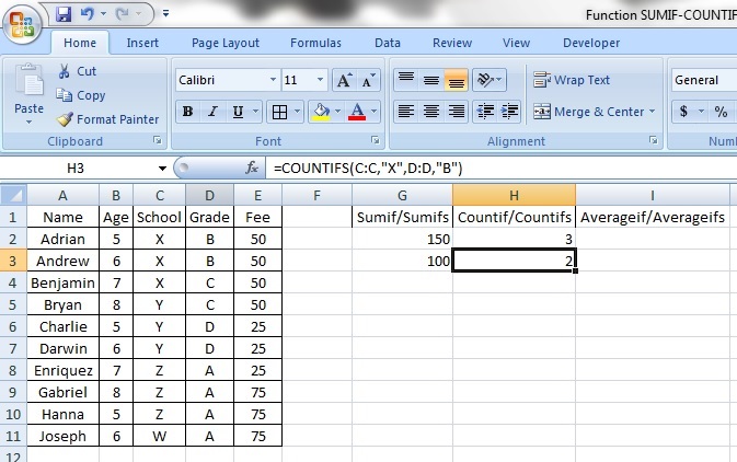
Let’s start with some data. Here we have a list of students, with the following columns – Name, Age, School, Grade and Fee. Now, let’s see what we can do.
SUMIF/SUMIFS
This function adds values together if they fulfil certain conditions that YOU specify!
SUMIF will only add values based on 1 specified condition
SUMIFS will add values based on more than 1 specified condition
Here’s an example. Let’s try to find out how much in fees students from school X pay:
=SUMIF(C:C,”X”,E:E)

Like all formulas, begin with ‘=’ and then the function SUMIF, with the contents framed by ‘(‘ and ‘)’.
How about the contents?
C:C refers to the data that contains the condition or criteria that would decide how the data is added together. In this case, this is the school the students go to.
“X”, is the criteria that we have specified. Hence, we are looking at column C:C and specifying “X” as the criteria. As it is a letter, remember to frame X with “ and “. If it was a number, there is no need of “ and “. So, we are looking only at students that go to school “X”.
E:E refers to the data we want added together, in this case, the fees that each student pays.
Hence, we want to add all the school fees together of all students that go to school “X”. So, we are adding the values contained in E:E that have the condition “X” in column C:C. In this case, the answer is $150.
SUMIFS
How about SUMIFS?
This function is very similar to SUMIF. Let’s see if we can find out how much fees students in school X that have B grades pay:
=SUMIFS(E:E,C:C,”X”, D:D,”B”)

Note how this is slightly different from SUMIF.
Like all formulas, begin with ‘=’ and then the function SUMIF, with the contents framed by ‘(‘ and ‘)’.
E:E refers to the data we want added together, in this case, the fees that each student pays.
C:C refers to the schools that the students have gone to. By specifying “X”, we are stating that we want only students from school “X”.
D:D refers to the grades that the students obtained and by specifying “B”, we are stating that we only want students with “B” grades.
Hence, we will get from the formula, the fees that all students from school “X” with “B” grades pay. In this case, $100.
Tip:
Remember that for SUMIFS, like COUNTIFS and AVERAGEIFS, you can add AS MANY CRITERIA AS YOU WANT!
COUNTIF/COUNTIFS
Like SUMIF and SUMIFS, COUNTIF counts values with 1 specified condition, while COUNTIFS counts values with more than 1 specified condition.
COUNTIF
Let’s see if we can find the number of students who attend school “Y”.
Here’s how it works:
=COUNTIF(C:C,”Y”)

C:C refers to the list where we want items counted. In this case, C:C refers to the schools that students go to.
“Y” refers to the item we want counted. This means that we want the number of students who attend school “Y”, the answer being 3.
COUNTIFS
Let’s see if we can find the number of students that attend school “X” and have gotten “B” grades:
=COUNTIFS(C:C,”X”,D:D,”B”)
Now, C:C and D:D refer to the lists where we want items counted, with “X” being the school attended and “B” being the attained grades.
Hence, we will get the number of students who have attended school “X” and attained the “B” grade, which is 2.
AVERAGEIF/AVERAGEIFS
Much the like the previous 2 functions, AVERAGEIF determines the average of items with 1 specified condition, while AVERAGEIFS, like its counterparts, determines the average of items with more than 1 specified conditions. They work in the same way too.
AVERAGEIF
Let’s find out the average of fees paid by students from school “Z”:
=AVERAGEIF(C:C,”Z”,E:E)
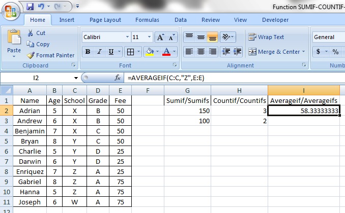
C:C refers to the list of schools, with “Z” being the condition specified. So we are looking at school “Z” specifically.
E:E refers to the items we want averaged, in this instance the fees paid. So we will get the average of fees paid by all students from school “Z”. The average being $58.33.
AVERAGEIFS
The final function we will look at today is the plural version of AVERAGEIF. AVERAGEIFS determines the average of items with more than 1 specified condition.
Let’s try to find out the average of fees paid by students from school “Y”, who have gotten “D” grades:
=AVERAGEIFS(E:E,C:C,”Y”,D:D,”D”)

E:E refers to the items we want averaged, in this instance the fees paid.
C:C refers to the list of schools, with “Y” being the condition specified. So we are looking at school “Y” specifically.
D:D refers to the grades that the students obtained and by specifying “D”, we are stating that we only want students with “D” grades.
With all that, we get the average of fees paid by all students from school “Y” who have attained a “D” grade. The result of that is $25.
Feeling mighty, yet?

Leave a comment