Aesthetics 3: Conditional Formatting

Aesthetics 3: Conditional Formatting

Time to learn: 10 minutes

Ever wish you could tell at a glance who your top performers are? Now you can!

Conditional formatting is an exciting aspect of Excel that allows you to change the way your spreadsheet LOOKS, based on the DATA entered.

Let’s have a look by starting with some data:

Here we have 12 colleagues and the total number of calls they have made from January to June.

Now, we will colour-code all the numbers to find out the top 3 and the bottom 3 in terms of performance each month.

Step 1: Select the ‘Home’ tab and highlight all the values in the ‘Jan’ column, like so.

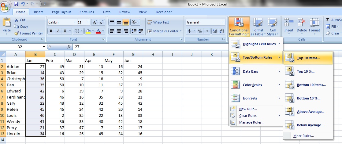
Step 2: Click on ‘Conditional Formatting’ and then select ‘Top/Bottom Rules’ and then ‘Top 10 items…’. Remember to ensure that all the values in the ‘Jan’ column are still highlighted.

Step 3: An option box will appear.  In the field that indicates ‘Format cells that rank in the TOP:’, enter the value 3.  This will mean that the conditional formatting will affect only the top 3 numbers.  If you enter 5, it will then affect the top 5.

Step 4: You can select how you want the cells to be formatted by selecting one of the options in the dropdown box on the right.  Here, we will choose ‘Light Red Fill with Dark Red Text’.

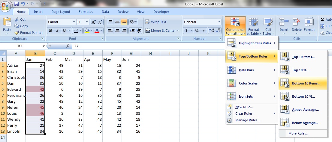
Now, the top 3 in ‘Jan’ have been highlighted in red!

Step 5: Now, follow step 1 to 3 again, but select ‘Bottom 10 items…’ instead.

Step 6: When the option box appears, enter 3 in the field that indicates ‘Format cells that rank in the BOTTOM:’.  For the formatting, we will choose ‘Yellow Fill with Dark Yellow Text’.

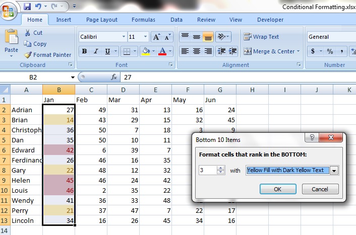
Step 7: Now the bottom 3 values are in yellow.

Nice.

Step 8: Now, to ensure that this formatting applies to all the months, select all the cells from B2 to B13 (this is the list of numbers for ‘Jan’) and right click.  Select ‘Copy’.

Step 9: Left click on the first cell with numbers in it in the ‘Feb’ column.  Right click and select ‘Paste Special’.

Step 10: Now, click on ‘Formats’.

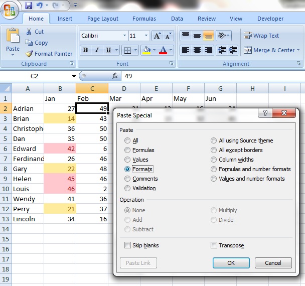
Step 11: Click ‘OK’ and you will see that the list of numbers in ‘Feb’ have been modified with the same conditional formatting as that in ‘Jan’.

Awesome.