Cells and Spreadsheets
Time to learn: 20 minutes
The foundation of each Excel file is called a SPREADSHEET. A spreadsheet is what you call all those rectangular boxes on your screen.

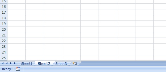
Most Excel files come with 3 spreadsheets once you open them, indicated by the 3 tabs at the bottom of the screen that say ‘Sheet 1’, ‘Sheet 2’ and ‘Sheet 3’.
Each of those little rectangular boxes within spreadsheets are called CELLS and are the primary building blocks we will be working with.
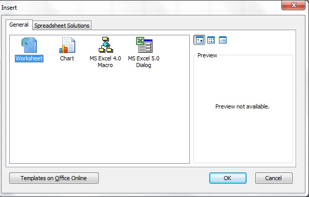
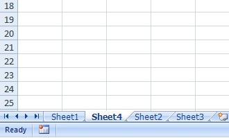
You may ADD spreadsheets by pointing at any of the sheet tabs, performing a right-click and then selecting ‘Insert’ and then selecting ‘Worksheet’;
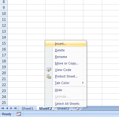
or ‘DELETE’, in which case, the spreadsheet DISAPPEARS!

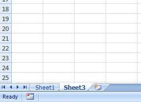
You can also RENAME your spreadsheet for reference later on by pointing to the sheet tab you want to rename, performing a right-click and then selecting ‘Rename’. The name of the sheet tab will darken and then you can enter the name of the sheet that you want. Alternatively, you can just perform a double left-click on the name of the sheet tab and the name of the sheet will darken. As before, you can now change the name of the sheet tab.


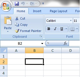
Have a look at the top most line of cells. You will see that there are grey boxes above them with letters in them. These are known as COLUMN labels. They exist so you can keep track of where your data is in a spreadsheet. Now observe the left most line of cells. Like column labels, the grey boxes with numbers in them are known as ROW labels and exist for the same purpose as column labels.
Think of the spreadsheet as a map and the COLUMNS being X-coordinates and the ROWS being Y-coordinates.
An easy way to remember what a column and row is in Excel is to use the following alphabetical association:
Ceiling (top most line of cells) = COLUMN
Left to Right (left most line of cells) = ROW
Please tell me that made it easier to understand?
If you’d like to know the location of a particular cell, all you have to do is left-click on a cell and its location, using the alphabetical COLUMN reference and the numerical ROW reference, a combination of the two will appear beside the formula bar. In this example, the selected cell with the dark border is located at ‘B2’.

Leave a comment