Do you need to compare results of an experiment or a marketing plan? Have you just changed the settings of your slot machines and aren’t sure whether the change resulted in a real difference in earnings? Have you just completed an intensive player promotion programme and need to find out whether it was effective?
Statistics has a simple way of calculating if the revenue before and after resulted in a real change in performance and also the probability that the change was a DIRECT result of the changes you made! This method is known as a T-Test.
A T-Test compares the averages of 2 sets of values and assesses how different the sets of data are. A companion to this is the R² measure of effect size, which calculates how much in terms of percentages that the results of your T-Test was affected directly by the change you implemented.
Here’s an example:
Casino A recently changed the settings of its slots machines and wants to find out if the change resulted in a positive change.
Here are the earnings of 5 machines BEFORE the change in settings and AFTER the change in settings:
Slot Before After
1 $10 $20
2 $14 $45
3 $12 $25
4 $8 $15
5 $16 $32
Now, we can see intuitively that the change was beneficial, but we normally don’t just compare such a small number – you are normally looking at hundreds or thousands of results. The results before and after changes may also not be so clearly different. So, how do you tell?
Step 1:
First, we calculate the average of each set of data. Let’s call them AVERAGE(Before) and AVERAGE(After).
AVERAGE(Before) = 10+14+12+8+16 / 5 = 12
AVERAGE(After) = 20+45+25+15+32 / 5 = 27.4
Step 2:
Now, we subtract each individual BEFORE result from each individual AFTER result to see what the difference is.
Slot After Before
1 $20 – $10 = $10
2 $45 – $14 = $31
3 $25 – $12 = $13
4 $15 – $8 = $7
5 $32 – $16 = $16
Step 3:
Now, we find the standard deviation of the differences. We find the standard deviation by the following:
1. Taking each value and subtracting it from the average of the differences:
10+31+13+7+16 / 5 = $15.4
10 – 15.4 = -5.4
31 – 15.4 = 15.6
13 – 15.4 = -2.4
7 – 15.4 = -8.4
16 – 15.4 = -0.6
2. Summing the square of each result
(-5.4)(-5.4) = 29.16
(15.6)(15.6) = 243.36
(-2.4)(-2.4) = 5.76
(-8.4)(-8.4) = 70.56
(-0.6)(-0.6) = 0.36
29.16+243.36+5.76+70.56+0.36 = 349.2
3. Divide the total by the total number of machines – 1.
349.2/4 = 87.3
4. Finally, square root the result.
SQRT(87.3) = 9.343446901
Standard Deviation of differences = 9.343446901
Step 4:
Now, we take AVERAGE(After) – AVERAGE(Before) and divide it by the standard deviation of differences, divided by the square root of the number of machines.
27.4 – 12 = 15.4
15.4 / (9.343446901 / SQRT(5))
15.4 / 4.178516483
T = 3.685518548
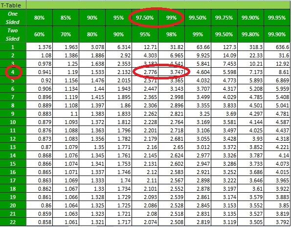
The T-statistic we get is 3.685518548. So what do we do with the T-statistic? This is the interesting part. We compare this to the T-table, which you can get off the internet.

We compare the T-statistic with the degrees of freedom (that is just a fancy way of saying the total number of samples -1. In our case, 5-1 = 4) and then get the probability percentage, which is between 2.5% (100% – 97.50%) – 1% (100% – 99%).
Which means that the probability of getting this result BY CHANCE is between 2.5% – 1%. This means that whatever you did, it worked.
Here’s the formula for a dependent T-test:
T = mean1 – mean2 / (standard deviation of the differences between sample1 and sample2 / sqrt(n))
We mentioned the R² measure of effect size as well. We use this to find out the percentage that this change in results was directly caused by the change in machine settings. We find this by taking the square of the T-statistic, divided by the square of the T-statistic added to the number of machines -1.
T² = (3.685518548)(3.685518548) = 13.58304696
R² = 13.58304696 / (13.58304696 + 4)
R² = 0.772508143 or 77.25%
So, now we know that the probability of this result being achieved due directly to the change is 77.25%.
Neat!
This may seem like a lot – so I’ve included a template for download that calculates the T-statistic and R² correlations for you when you enter in sample data. Just follow the instructions and you’ll get it.
https://drive.google.com/file/d/0B1pEq2dN7H9ANmhfZzAwOWFJS3M/view?usp=sharing
You can use the T-Test for anything, really. You could compare the test scores of your nephew before and after he’s been fed an all vegetable diet, the effectiveness of a marketing plan based on the amount spent by a specific group of clients before and after – you get the idea.
Have fun!

Leave a comment