Concepts 7: Compare How Different Areas of Your Casino are doing using an Independent T-Test!

What if you wanted to compare different areas with different numbers of machines on your gaming floor? What if you wanted to know if a certain area was receiving more profit than another?

In a previous post, we looked at how we can measure the effects of a change in machine settings on the earnings of a group of slot machines, using a dependent T-Test.

For the post, see here: https://excelpunks.com/comparisons-using-t-tests/

If you recall, a dependent T-test compares the differences in means of data with identical sample sizes before and after treatment – our data being the earnings of a slot machine and the treatment being a change in settings.

An independent T-test allows us to compare data sets with different numbers of samples to determine if they are statistically different.

Here’s an example:

A casino has 2 slot zones, Zone 1, with 5 machines and Zone 2, with 10 machines.  We want to find out if one area is earning more than another.

Here’s the data.

Zone 1 Machines	Earnings	Zone 2 Machines	Earnings
1	$16	1	$8
2	$12	2	$10
3	$11	3	$15
4	$20	4	$15
5	$15	5	$14
		6	$15
		7	$12
		8	$8
		9	$13
		10	$13

Step 1:

Calculate the mean earnings of each zone.

Zone 1 mean = (16 + 12 + 11 + 20 + 15) / 5 = $14.80

Zone 2 mean = (8 + 10 + 15 + 15 + 14 + 15 + 12 + 8 + 13 + 13) / 10 = $12.40

Step 2:

Subtract each machine’s individual earnings from their respective zone means and square the result.

Zone 1 Machines	Earnings	Earnings – Zone 1 Mean	Square	Zone 2 Machines	Earnings	Earnings – Zone 2 Mean	Square
1	$16	16-14.80 = 1.2	$1.44	1	$8	8-12.40 = -4.4	$19.36
2	$12	12-14.80 = -2.8	$7.84	2	$10	10-12.40 = -2.4	$5.76
3	$11	11-14.80 = -3.8	$14.44	3	$15	15-12.40 = 2.6	$6.76
4	$20	20-14.80 = 5.2	$27.04	4	$15	15-12.40 = 2.6	$6.76
5	$15	15-14.80 = 0.2	$0.04	5	$14	14-12.40 = 1.6	$2.56
				6	$15	15-12.40 = 2.6	$6.76
				7	$12	12-12.40 = -0.4	$0.16
				8	$8	8-12.40 =  -4.4	$19.36
				9	$13	13-12.40 = 0.6	$0.36
				10	$13	13-12.40 = 0.6	$0.36

Step 3:

Now add the results together and divide them by the total number of samples -2.

Zone 1 = 1.44 + 7.84 + 14.44 + 27.04 + 0.04 = 50.80

Zone 2 = 19.36 + 5.76 + 6.76 + 6.76 + 2.56 + 6.76 + 0.16 + 19.36 + 0.36 + 0.36 = 68.20

50.80 + 68.20 = 119

119 / 5+10-2 = 119/13 = 9.15 (this is known as the Pooled Variance)

Step 4:

Divide the pooled variance by the respective sample sizes of the 2 zones, add the result and finally square root that.

(9.15 / 5) + (9.15/10) = 1.83 + 0.92 = 2.75

Square Root 2.75 = 1.657

Step 5:

Now, we take the difference of the means for Zone 1 and 2 and divide it by 1.657.  This is known as your T-statistic.

T = 14.80 – 12.40 / 1.657 = 2.40 / 1.657 = 1.448267583 or 1.448

Step 6 (Finally):

Compare the T-statistic with the T-table.  Looking at this table, we get our degrees of freedom, or df, by subtracting 2 from 5+10 = 13.  Now, we will find our T-statistic on this table.

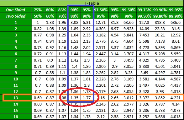
We see that our T-statistic of 1.448 is between 90% – 95% on a one-tailed test.  This means that we are between 90% – 95% sure that from this sample data, Zone 1’s earnings are higher than Zone 2’s earnings.

Perhaps you might want to place more machines in Zone 1 then?

Here’s the formula for an independent T-test:

T = mean₁ – mean₂ / sqrt((pooled variance / n₁) + (pooled variance / n₂))

Here’s a spreadsheet that allows you to compare data using the Independent T-test.  Just paste your data in the columns A and B and click ‘Compute’!

https://drive.google.com/file/d/0B1pEq2dN7H9Aa3RTdng3b1d1M00/view?usp=sharing