Concepts 6: Check for a Biased Wheel, or a Dealer’s biased spin with Chi Square Tests

Chi²

The Chi² distribution tests for the difference between the observed and the expected in terms of frequencies.  We can apply this to a simple example:

In double-zero roulette, we have 38 numbers and the expected probability of any one of these numbers appearing is 1/38 or 0.026316 or 2.6316%.  Now, assuming you track all the results that appear on your roulette tables, you’d be able to check for biased wheels or even if your dealers have developed the muscle memory to spin at a regular area of the wheel.

As with all things probable, do note that nothing is impossible.  It may be unlikely, but never impossible.  Always correlate your findings with footage from surveillance.

Number	Probability
0-0	0.026316
0	0.026316
1	0.026316
2	0.026316
3	0.026316
4	0.026316
5	0.026316
6	0.026316
7	0.026316
8	0.026316
9	0.026316
10	0.026316
11	0.026316
12	0.026316
13	0.026316
14	0.026316
15	0.026316
16	0.026316
17	0.026316
18	0.026316
19	0.026316
20	0.026316
21	0.026316
22	0.026316
23	0.026316
24	0.026316
25	0.026316
26	0.026316
27	0.026316
28	0.026316
29	0.026316
30	0.026316
31	0.026316
32	0.026316
33	0.026316
34	0.026316
35	0.026316
36	0.026316

Let’s say we have tracked 1,000 spins on a particular roulette table.  We are thus expecting that each number would have appeared 1,000 x 0.026316 = 26.316 times.  Do note that you would have to give or take an allowance of -1σ to 1σ based on the central limit theorem.

Here are our results based on 1,000 spins:

Number	Probability	Expected	Occurrence
00	0.0263	26.3158	13
0	0.0263	26.3158	32
1	0.0263	26.3158	32
2	0.0263	26.3158	27
3	0.0263	26.3158	39
4	0.0263	26.3158	20
5	0.0263	26.3158	33
6	0.0263	26.3158	23
7	0.0263	26.3158	10
8	0.0263	26.3158	36
9	0.0263	26.3158	29
10	0.0263	26.3158	17
11	0.0263	26.3158	38
12	0.0263	26.3158	14
13	0.0263	26.3158	11
14	0.0263	26.3158	25
15	0.0263	26.3158	20
16	0.0263	26.3158	16
17	0.0263	26.3158	11
18	0.0263	26.3158	12
19	0.0263	26.3158	28
20	0.0263	26.3158	17
21	0.0263	26.3158	45
22	0.0263	26.3158	24
23	0.0263	26.3158	43
24	0.0263	26.3158	25
25	0.0263	26.3158	10
26	0.0263	26.3158	21
27	0.0263	26.3158	43
28	0.0263	26.3158	23
29	0.0263	26.3158	42
30	0.0263	26.3158	30
31	0.0263	26.3158	18
32	0.0263	26.3158	45
33	0.0263	26.3158	40
34	0.0263	26.3158	41
35	0.0263	26.3158	17
36	0.0263	26.3158	30

To find the Chi² value, the following formula applies:

Sum of all (observed values – expected values)² / expected values

This works out to be the following:

Number	Probability	Expected	Occurrence	Observed – Expected	Observed – Expected2	Observed – Expected2/Expected	Sum
1	0.03	26.32	13	-13.32	177.31	6.74	172.984
1	0.03	26.32	32	5.68	32.31	1.23
1	0.03	26.32	32	5.68	32.31	1.23
2	0.03	26.32	27	0.68	0.47	0.02
3	0.03	26.32	39	12.68	160.89	6.11
4	0.03	26.32	20	-6.32	39.89	1.52
5	0.03	26.32	33	6.68	44.68	1.70
6	0.03	26.32	23	-3.32	10.99	0.42
7	0.03	26.32	10	-16.32	266.20	10.12
8	0.03	26.32	36	9.68	93.78	3.56
9	0.03	26.32	29	2.68	7.20	0.27
10	0.03	26.32	17	-9.32	86.78	3.30
11	0.03	26.32	38	11.68	136.52	5.19
12	0.03	26.32	14	-12.32	151.68	5.76
13	0.03	26.32	11	-15.32	234.57	8.91
14	0.03	26.32	25	-1.32	1.73	0.07
15	0.03	26.32	20	-6.32	39.89	1.52
16	0.03	26.32	16	-10.32	106.42	4.04
17	0.03	26.32	11	-15.32	234.57	8.91
18	0.03	26.32	12	-14.32	204.94	7.79
19	0.03	26.32	28	1.68	2.84	0.11
20	0.03	26.32	17	-9.32	86.78	3.30
21	0.03	26.32	45	18.68	349.10	13.27
22	0.03	26.32	24	-2.32	5.36	0.20
23	0.03	26.32	43	16.68	278.36	10.58
24	0.03	26.32	25	-1.32	1.73	0.07
25	0.03	26.32	10	-16.32	266.20	10.12
26	0.03	26.32	21	-5.32	28.26	1.07
27	0.03	26.32	43	16.68	278.36	10.58
28	0.03	26.32	23	-3.32	10.99	0.42
29	0.03	26.32	42	15.68	245.99	9.35
30	0.03	26.32	30	3.68	13.57	0.52
31	0.03	26.32	18	-8.32	69.15	2.63
32	0.03	26.32	45	18.68	349.10	13.27
33	0.03	26.32	40	13.68	187.26	7.12
34	0.03	26.32	41	14.68	215.63	8.19
35	0.03	26.32	17	-9.32	86.78	3.30
36	0.03	26.32	30	3.68	13.57	0.52

So, our Chi² is 172.984.

We now look for this figure on the chi² table.  The numbers at the top are the probability percentages and the column on the left marked df just refer to the number of categories you are looking at -1.  In our case, it’ll be 38-1 or 37.  We’ll look at df=40 as it is the closest to 37.

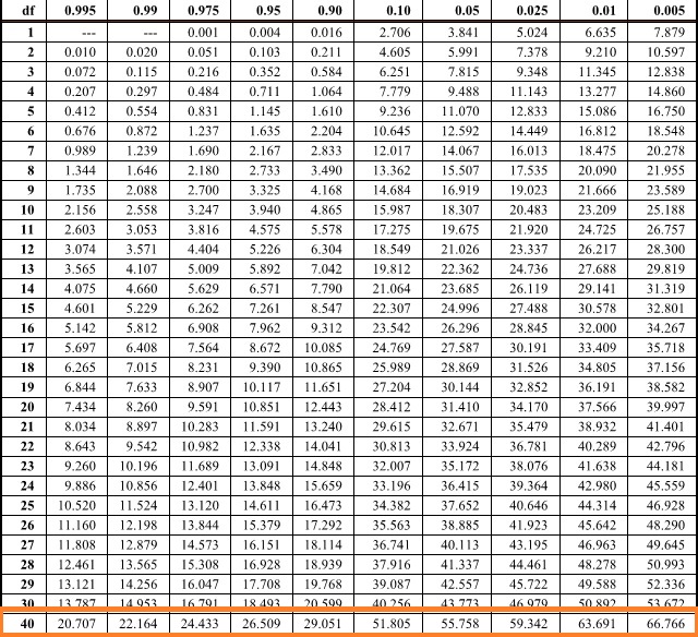
Our chi value of 172.984 exceeds all the probabilities on the chi² table, which means that there is DEFINITELY a PROBABILITY of the wheel or the dealer being or doing something out of the ordinary.

So, which ones?

Residuals

We can look at each number from 00 – 36 and identify which ones were out of the ordinary.  We do this by calculating what is called a residual.  This is just fancy for how different each result is from the expected.  Here’s the formula:

Observed result – Expected result / Square root (Expected result)

So, for 00, the formula would translate to:

13 – 26.32 / square root(26.32) = -13.32/5.129 = -2.59573

Number	Probability	Expected	Occurrence	Observed – Expected	Residual
0-0	0.03	26.32	13	-13.32	-2.59573
0	0.03	26.32	32	5.68	1.108057
1	0.03	26.32	32	5.68	1.108057
2	0.03	26.32	27	0.68	0.133377
3	0.03	26.32	39	12.68	2.472608
4	0.03	26.32	20	-6.32	-1.23117
5	0.03	26.32	33	6.68	1.302993
6	0.03	26.32	23	-3.32	-0.64637
7	0.03	26.32	10	-16.32	-3.18053
8	0.03	26.32	36	9.68	1.8878
9	0.03	26.32	29	2.68	0.523249
10	0.03	26.32	17	-9.32	-1.81598
11	0.03	26.32	38	11.68	2.277672
12	0.03	26.32	14	-12.32	-2.40079
13	0.03	26.32	11	-15.32	-2.9856
14	0.03	26.32	25	-1.32	-0.25649
15	0.03	26.32	20	-6.32	-1.23117
16	0.03	26.32	16	-10.32	-2.01092
17	0.03	26.32	11	-15.32	-2.9856
18	0.03	26.32	12	-14.32	-2.79066
19	0.03	26.32	28	1.68	0.328313
20	0.03	26.32	17	-9.32	-1.81598
21	0.03	26.32	45	18.68	3.642223
22	0.03	26.32	24	-2.32	-0.45143
23	0.03	26.32	43	16.68	3.252351
24	0.03	26.32	25	-1.32	-0.25649
25	0.03	26.32	10	-16.32	-3.18053
26	0.03	26.32	21	-5.32	-1.03624
27	0.03	26.32	43	16.68	3.252351
28	0.03	26.32	23	-3.32	-0.64637
29	0.03	26.32	42	15.68	3.057415
30	0.03	26.32	30	3.68	0.718185
31	0.03	26.32	18	-8.32	-1.62105
32	0.03	26.32	45	18.68	3.642223
33	0.03	26.32	40	13.68	2.667544
34	0.03	26.32	41	14.68	2.86248
35	0.03	26.32	17	-9.32	-1.81598
36	0.03	26.32	30	3.68	0.718185

All the residuals are now in terms of σ!  If you recall, the central limit theorem infers that all data should fall within the -3σ to 3σ region in relation to the mean.

The majority of outcomes would occur within the -1σ to 1σ region.  So a reading of -2.59573 means that the number 00 has been occurring less times than expected.

Conversely, a reading of 3.642223 for number 32, indicates that the number 32 has occurred 3.642223σs more than the mean.  Definitely worth some time investigating.