Functions 3: IFERROR

Function: IFERROR

Time to learn: 10 minutes

Ever wanted to have a clean looking formula that cuts out all the #N/As, #VALUEs and #REFs?

Today, we’ll look at a function that does just that.

The IFERROR function behaves like an add-on function and can be used easily in conjunction with any other formula.

Let’s look at a simple formula:

=A2+B2

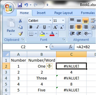
Let’s examine the contents.

A2 refers to the contents of the cell A2, which are numbers.

B2 refers to the contents of cell B2. You can see that some of the cells in column B are numbers and some are words.

We know that simply adding numbers with ‘+’ works fine, but doesn’t work when adding numbers and words together. So we are expecting it to give us a #VALUE, which it does.

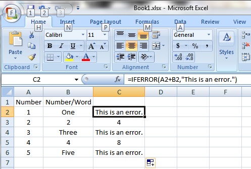
BUT, if you hate seeing that, we can add the IFERROR function – which is simply a value that the function gives you if the result of the original formula is an error, hence IFERROR.

Here’s an example:

=IFERROR(A2+B2,”This is an error.”)

Let’s look at the structure of the IFERROR function.

Like all formulas, we begin with an “=” and then the text of the function, IFERROR, with all the contents framed in a ‘(‘ and ‘)’.

A2 and B2 refer to the contents.

The IFERROR function comes before the initial formula of A2 + B2 and we also see that after the initial formula, we have added the text “This is an error.”.

What we have done is to insert the IFERROR function, making it a part of the A2 + B2 formula, so that if the result is some form of error, the cell will show the text, “This is an error.”.

You can add the IFERROR function to any other formula, so it is very versatile.