Functions 7: SUM, COUNT & AVERAGE

Function: SUM, COUNT & AVERAGE

Time to learn: 20 minutes

Now, let’s look at some mathematical expressions.

As you might have guessed, the 3 functions we are looking at today compute values by either SUMMING, COUNTING or AVERAGING them.

SUM

Here’s an example:

=SUM(1,2,3,4,5)

Now, what we’ve done is add the numbers 1 through 5 together to give us 15. Pretty easy, yeah?  What’s better is that we can use SUM to add the contents of cells together too.

Here’s an example:

=SUM(A1:A20)

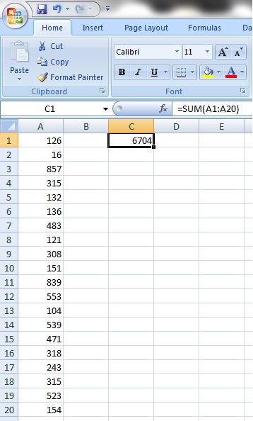
Now, here we’ve performed a SUM function on cells A1 through to A20 to give us 6704. You can do this by entering the “=SUM(“ and then clicking on the first cell you want to include into the formula and then holding the left mouse button and dragging it down to the last cell you want to include in the formula, then adding the closing “)”. This works for the other formulas in this post too.

You can also just select the whole column (or row if you’d like) if there are too many numbers by moving your mouse pointer to the column label of the column where all your numbers are and doing a left-click, like this:

=sum(A:A)

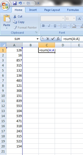
Notice that the blue lines bordering the selected cells now go into INFINITY and BEYOND. Be careful, though, as selecting the whole column now selects EVERYTHING in the column. Which may not be what you want to do.

Here’s something extra:

Let’s say that you wanted to add a column of values but some of the values contain text. Let’s try this first with the simple ‘+’ sign:

=A1+A2+A3+A4

Doh! An error.  Notice that when using the ‘+’ sign, only numerical values can be calculated.  BUT, now let’s try this with the SUM function:

=SUM(A1:A4)

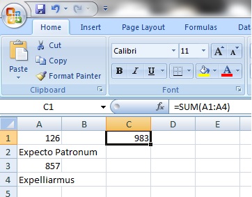
Whoa…that’s what I’m talking about. The SUM function ignores text and goes straight for the numbers, giving you the value of all the numbers added together.

COUNT / COUNTA

Yes, you guessed it, this function performs a count of how many items there are in a list of items, like so:

=COUNT(A1:A4)

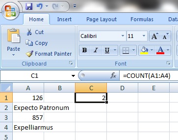
What? What happened?  Isn’t it supposed to give 4?  Well, COUNT works in a way that only counts numerical values.  Damn.  BUT, now we can use the COUNTA function, that counts ANYTHING in a cell:

=COUNTA(A1:A4)

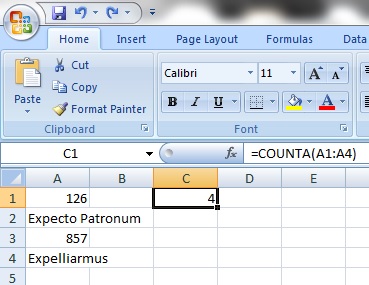
Isn’t that COOL or what?

AVERAGE / AVERAGEA

This function gives you the average of a set of numbers. Here’s an example:

=AVERAGE(A1:A4)

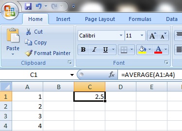
All fine and good when there are only numbers in the list. How about when there is a text value?

Whoa, what the hell? Notice that now instead of dividing the sum of all the numerical values by 4 items, AVERAGE divides the sum of the numerical values by the TOTAL number of numerical items, which is now 3, hence you get 2.66667, instead of 2 as you might expect.

Now, just like COUNTA, let’s add an A to AVERAGE. Here’s an example:

=AVERAGEA(A1:A4)

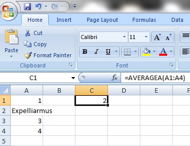
Now, we see that the sum of all the numerical values, 8, is now divided by ALL items in the list, regardless of what the cell contents are, giving us the value of 2.