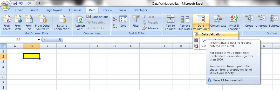
Basics 5: Paste Special
Time to learn: 20 minutes
The Paste Special function allows you to easily transfer data, formulas, formats or even perform mathematical operations just by using good old copy and paste!
This aspect of Excel seldom gets much attention as most do not understand how it works. That is going to change today.
Remember that you always start with some data you need to copy first and then proceed to paste it in another location in a special format that you decide on – that is the principle of the Paste Special function.
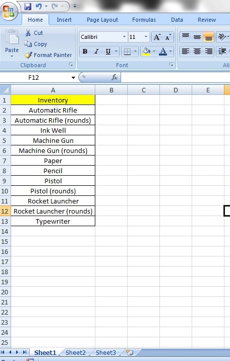
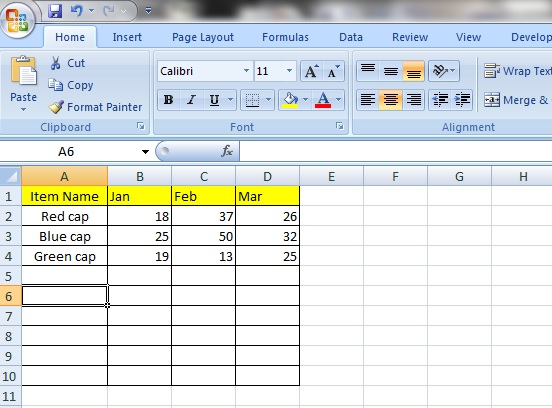
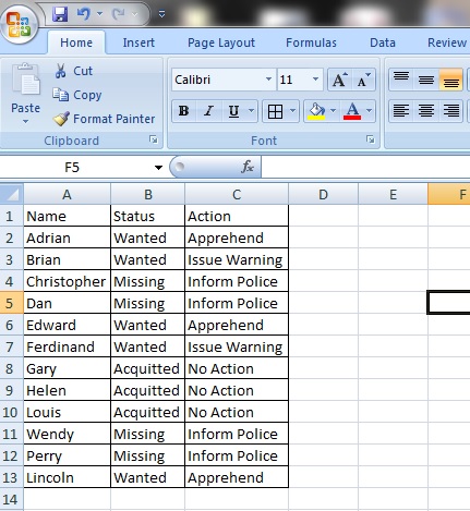
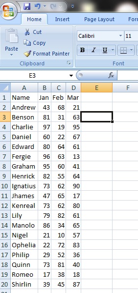
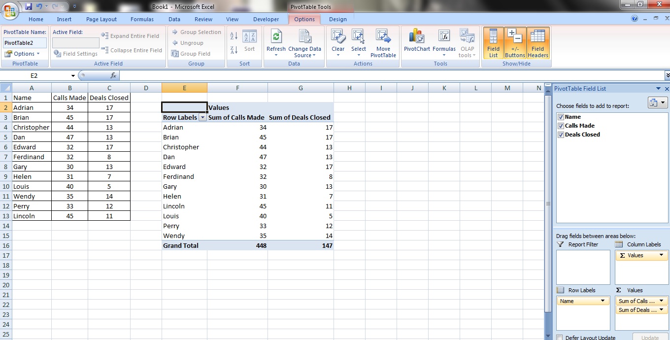
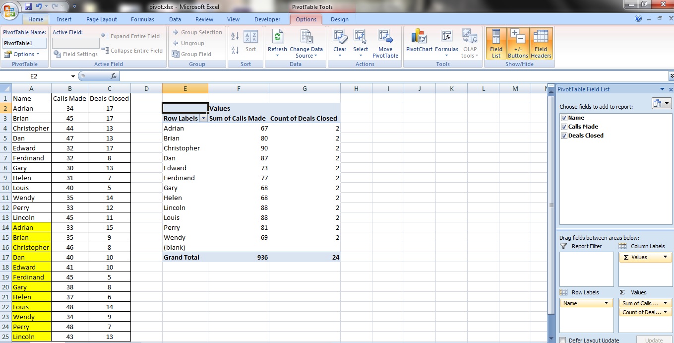
Let’s start with some data.
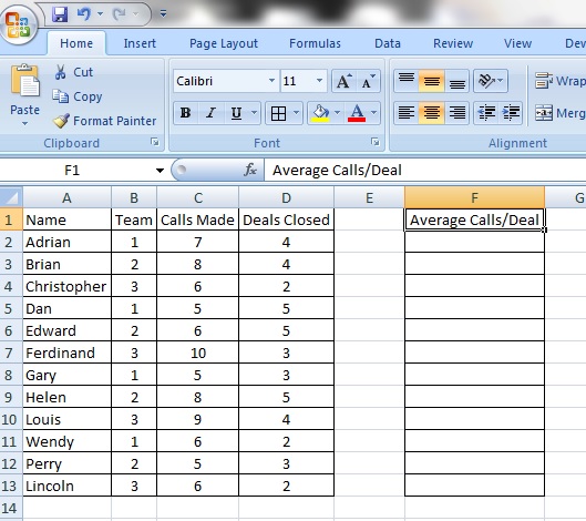
Here we have 12 colleagues grouped into 3 teams and their call records, including how many deals they have closed.

Mathematical Operations
Step 1:
Let’s find out how many calls on average it takes to close a deal for each of them. Let’s create a column called ‘Average Calls/Deal’.

Step 2:
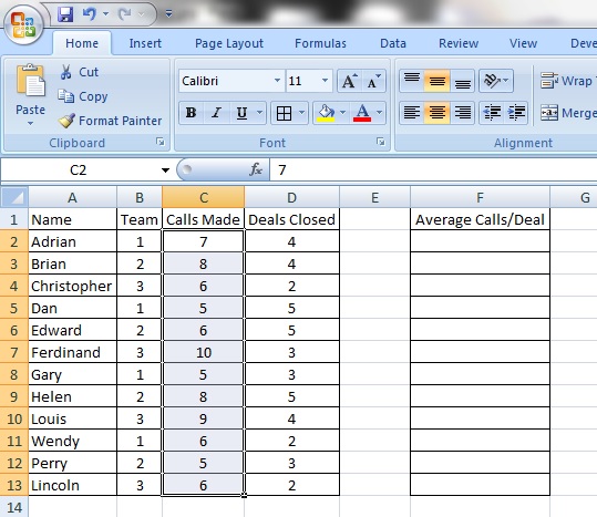
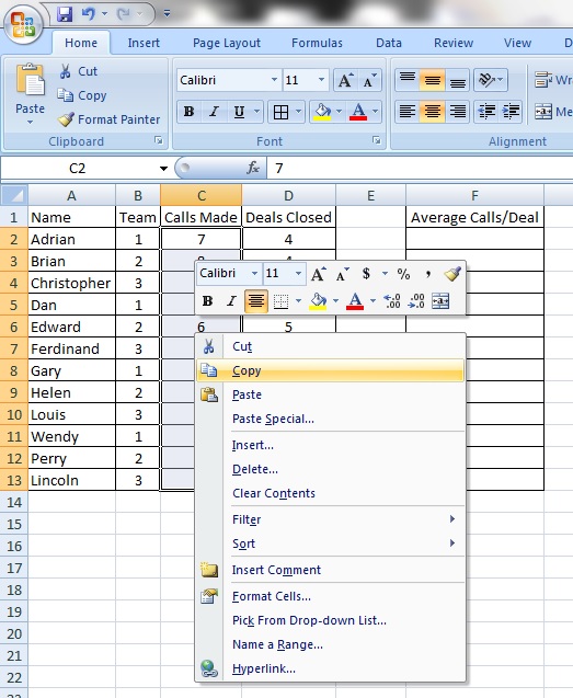
Highlight cells C2 to C13 – this cell reference contains the list of the number of calls made per person.

Now, with your cursor still within the cell reference C2 to C13, perform a right click and click on ‘Copy’. You can also use the Ctrl + C shortcut.

You should immediately see a line of running dashes around your selection – this is Excel’s way of saying that the cells have been selected for copying.
Step 3:

Paste the selection onto the ‘Average Calls/Deal’ column by right clicking on cell F2 (the first cell of the column ‘Average Calls/Deal’) and selecting ‘Paste’. You can also use the Ctrl + V shortcut.
Step 4:
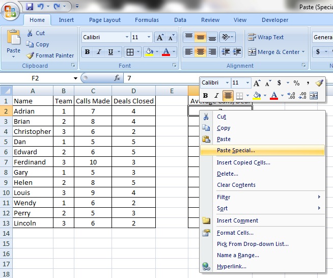
Copy the cells D2 to D13 – this cell reference contains the list of deals closed by each person. With your cursor still within the cell reference D2 to D13, perform a right click and click on ‘Copy’. You can also use the Ctrl + C shortcut.

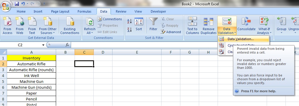
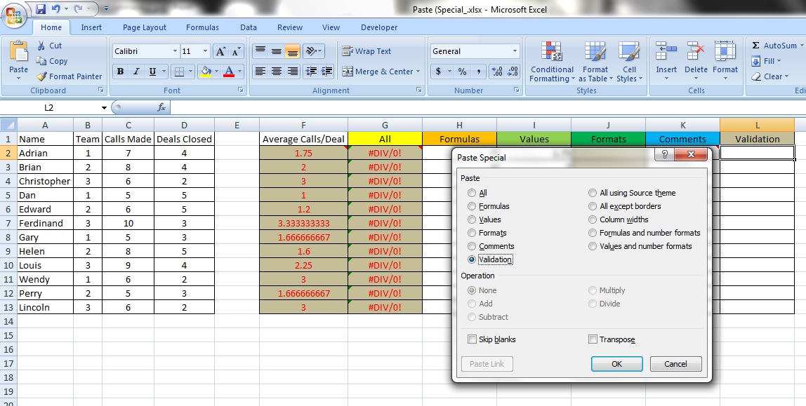
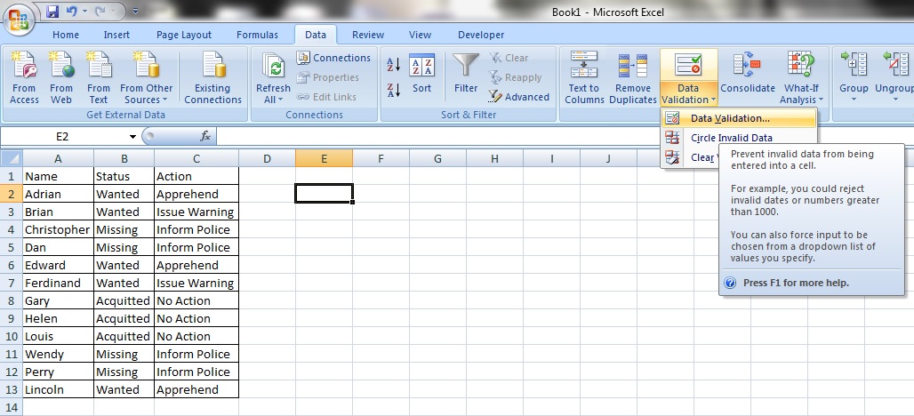
Ensuring that the cells in D2 to D13 are still selected, right click on the cell F2 and select ‘Paste Special’.
Step 5:
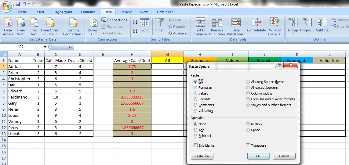
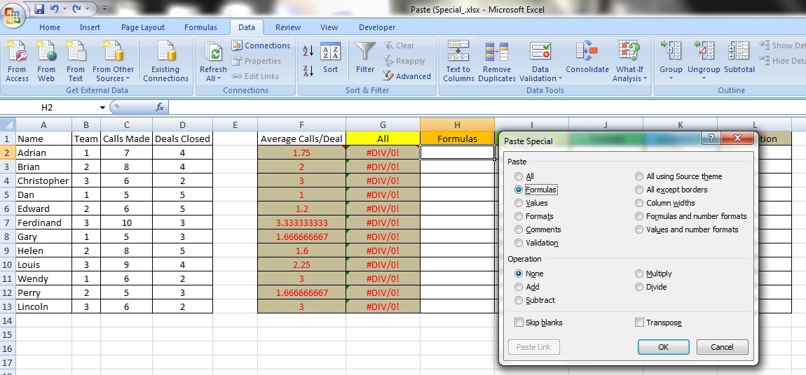
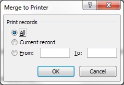
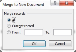
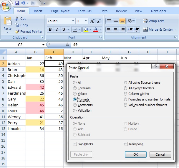
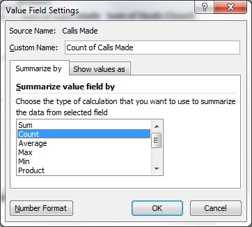
You will see an option box like this.

Under ‘Operation’, click on ‘Divide’ and click ‘OK’.

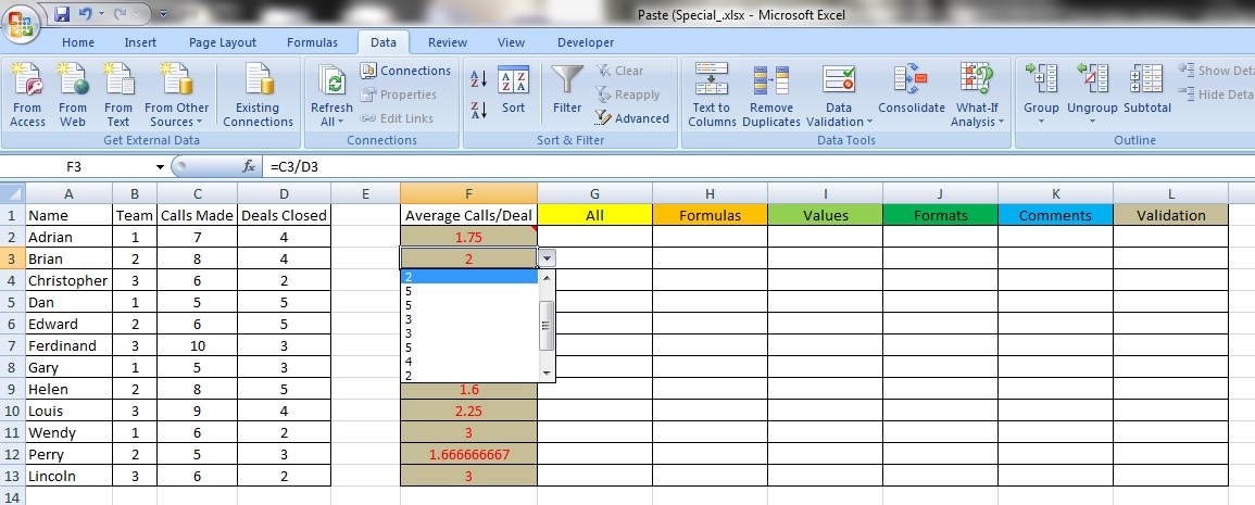
Now, you will see that all your colleagues’ call numbers have been divided by the number of deals they have closed per person.
Tip:
You would have noticed in the option box earlier under ‘Operation’ that there are other mathematical functions like ‘Add’, ‘Subtract’ and ‘Multiply’. That is exactly what it does. By copying and then using the ‘Paste Special’ function, you can add, subtract, multiply or divide a selection of numbers in a cell destination by the values you have copied instantly.
Paste Special
This section deals with the more interesting aspects of ‘Paste Special’.
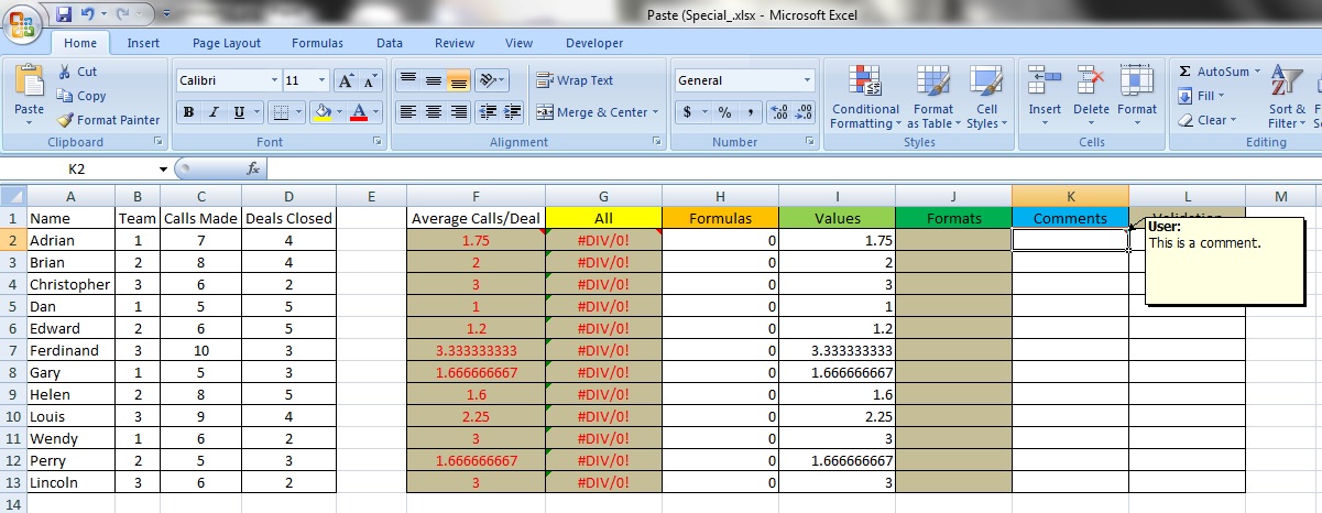
Notice in the ‘Paste Special’ option box under ‘Paste’, the 6 options – ‘All’, ‘Formulas’, ‘Values’, ‘Formats’, ‘Comments’ and ’Validation’.
I’ve created column titles for each one of these options to show you how they work.

Now, I’ve done a few things with the column ‘Average Calls/Deal’.
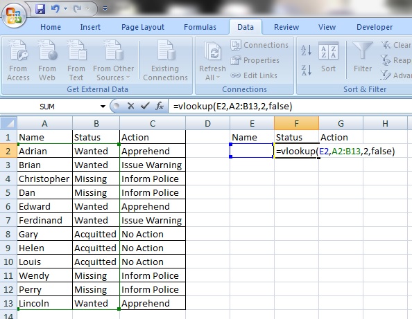
- Notice that when the cells are selected, they have a formula ‘=C2/D2’ – all of them have that, referencing cells in the ‘Calls Made’ and ‘Deals Closed’ columns and dividing the ‘Calls Made’ by the ‘Deals Closed’.

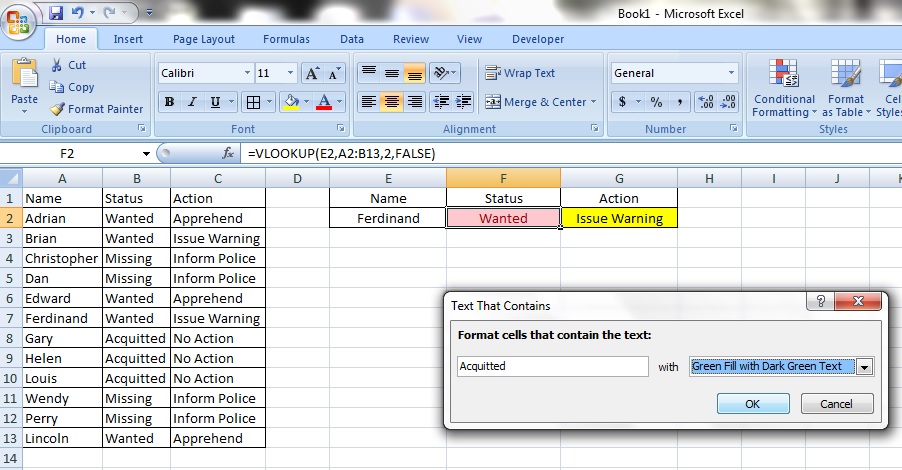
- Notice that the cell and text colour have been changed.
- There is also a comment in cell F2.

You can insert comments into cells by right clicking on the cell and selecting ‘Insert Comment’. Comments are free text boxes that you can use to contain information about a cell without affecting its contents.
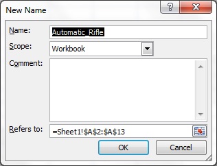
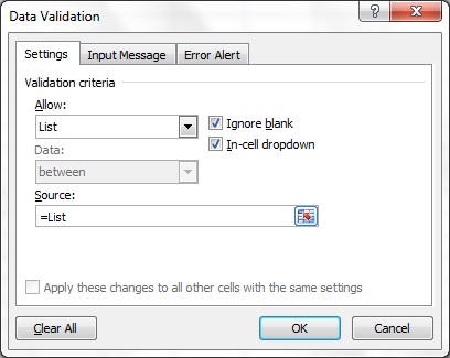
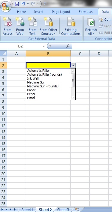
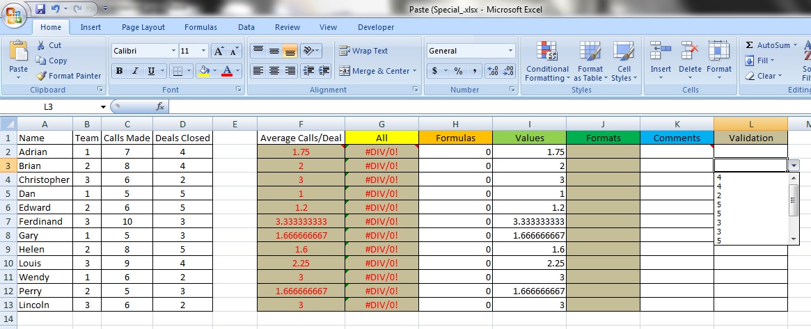
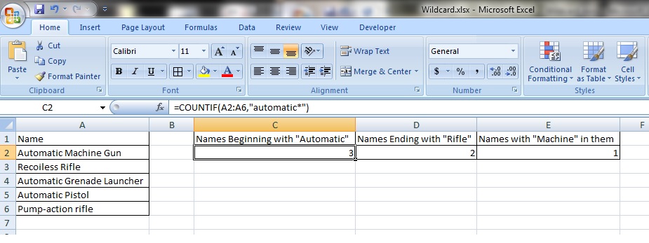
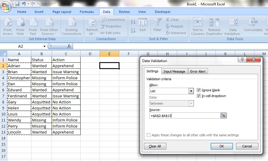
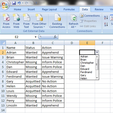
- In cell F3, I have also created a data validation list.

You can get more information on how to do this under Aesthetics 1: Dropdown Lists (Data Validation). This is just to illustrate the Paste Special function, though.
Step 1:
To illustrate what the 6 options, ‘All’, ‘Formulas’, ‘Values’, ‘Formats’, ‘Comments’ and ’Validation’ do, we will copy the whole cell selection from F2 to F13 and copy and Paste Special on each column, using one of the Paste functions.
All

Notice that every aspect has been copied over – formulas, formats, the comment and the data validation.

So what’s with the error messages?
Notice that when we copied over the cells F2 to F13, their contents contained the formulas ‘=C2/D2’? Now, the formula has moved 1 complete column to the right to cell ‘=D2/E2’ or ’=D3/E3’.
Why?
Because when we did a copy and Paste Special ‘All’ 1 column to the right, all the cell references moved as well in exactly the same way.
This is part of how Excel ‘intelligently’ tries to assist us. Don’t worry about this, though, as we expected this to occur.
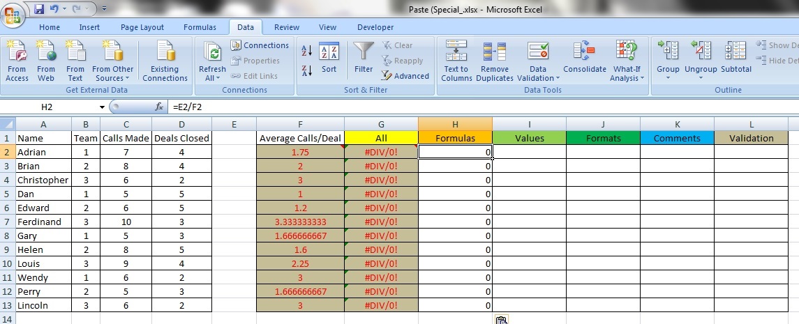
Formulas

Notice that only the formulas within each cell have been copied. Notice also that the formulas now indicate ‘=E2/F2’.

As with Paste Special ‘All’, whenever formulas are copied, they are moved exactly the same number of rows or columns and in the same direction.
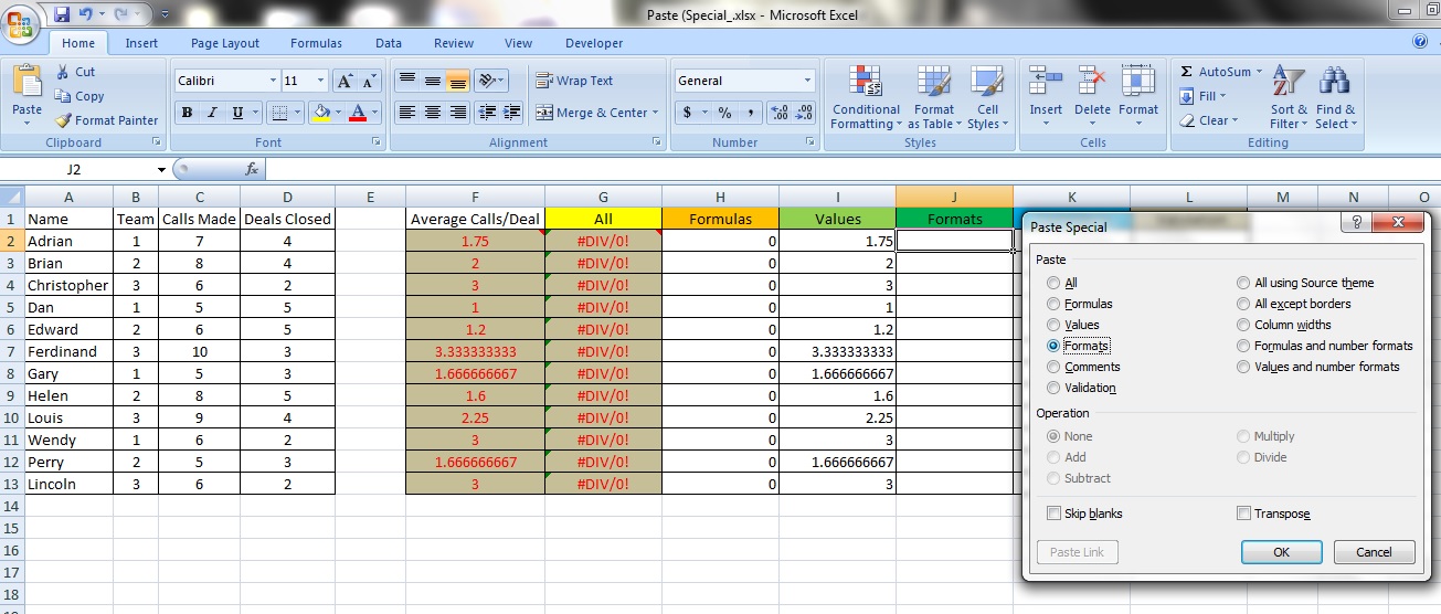
Values

Now, notice that only the values in the cells have been copied over?

There are no formulas, formatting, comments or data validation lists. This is for when you just want the results of the cells copied, nothing more.
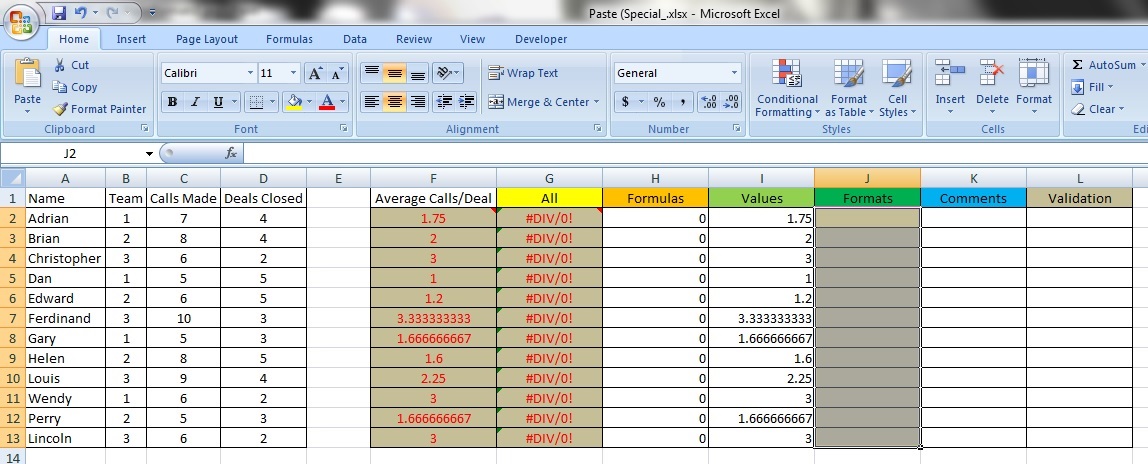
Formats

Observe that only the aesthetic formatting has been copied.

The cells are grey and if you type in any text, they will be red, like the original list. If you have applied Conditional Formatting to the cells, they will be carried over as well.
Comments

Notice that only the comment has been copied over.

Nothing more.
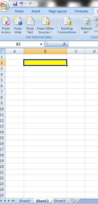
Validation

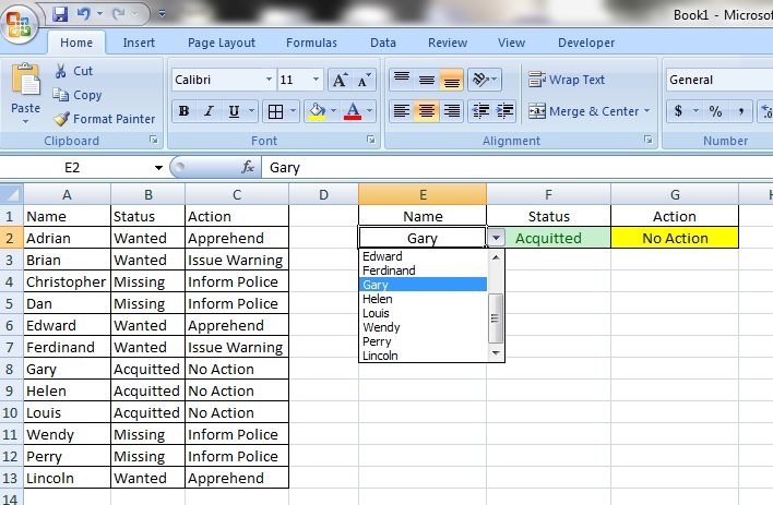
Notice that only the data validation list has been copied over.

Nothing more.
The remaining options are variations of those we have looked at.
All using Source Theme copies the theme of your cells, should you have applied one.

You can access the Themes function by going to the ‘Page Layout’ tab and selecting ‘Themes’. This changes the overall look of your Excel spreadsheets.
All except borders is similar to All, except that the borders are not copied.
Column widths only copies the exact width of the original cells – more aesthetic than anything.
Formulas and number formats – copies only the formulas (remember that the cell references move accordingly) and the formatting of the contents of the cells.
Values and number formats – copies only the value of the contents of the cell; not its formula, and the formatting of the contents of the cells.