Data Processing 2: Pivot Tables
Time to learn: 20 minutes
Have tonnes of data that you can’t make sense of? Need a fast way to organise and view your 10,000 cell spreadsheet? Then, pull that rabbit out of your hat with pivot tables!
A pivot table compiles and summarises all the information in a spreadsheet into a table that you can manipulate easily. Saves you time and makes you look incredible!
The pivot table is an awesome function and helps you do many things at once!
Step 1:
Let’s start with some data.
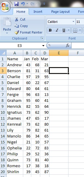
Here we have 19 colleagues and the number of sales they have completed from January to March.
Now, what if we want to count the total sales for all of them per month?
Step 2:
Now, click on any cell that has our data in it (meaning anywhere from cells A1 to D20) and then click on the ‘Insert’ tab and select ‘Pivot Table’.

Step 3:
An option box will appear. Now, notice that in the box below ‘Select a table or range’, you will see the cell reference Sheet1!$A$1:$D$20.
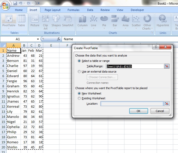
Notice that this is exactly the cell reference of our list of names and sales per month from January to March?
This means that the pivot table will use all the information from cells A1 to D20. Neat!
Tip:
You can change this reference by selecting a new range of cells if you want. This allows for changing the contents of your table.
Step 4:
Now, we move to the option ‘Choose where you want the PivotTable to be placed’.
You have 2 options.
Option 1:
‘New Worksheet’ automatically creates a new tab with the pivot table once you click ‘OK’, like so.
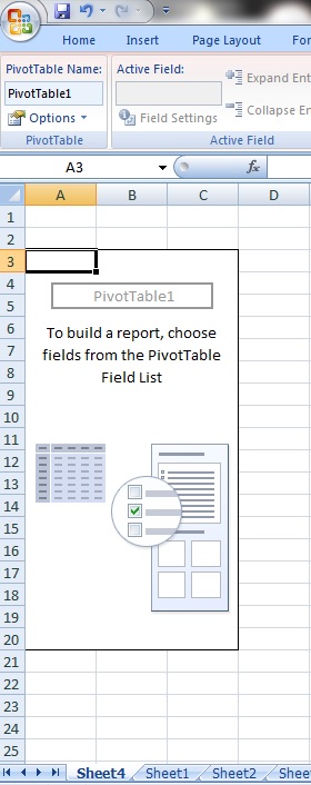
Notice that a new sheet, ‘Sheet 4’, has been created with the pivot table on the left side of the screen and the options on the right side of the screen.
Option 2:
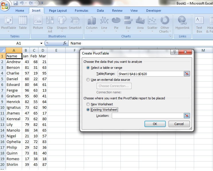
‘Existing Worksheet’ allows you to place the pivot table on the same sheet as your data. In this case, we have selected cell F2, which becomes bordered in dotted lines.

In the ‘Location’ box, you now see the cell reference Sheet1!$F$2, which refers to the location where we want the pivot table placed – in cell F2!
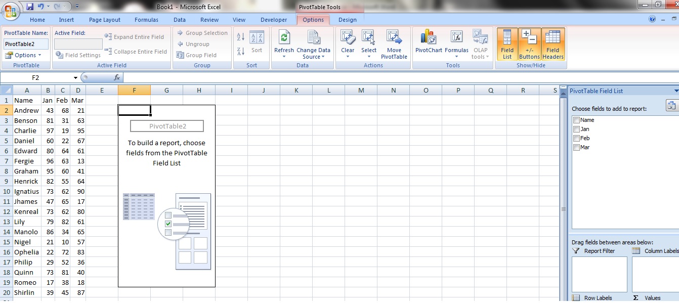
Clicking ‘OK’ creates a pivot table on the same sheet, with several options boxes on the right side.
Step 5:
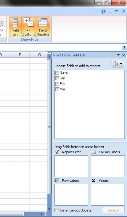
Now, notice that the titles of the data (the first cell of each column), ‘Name’, ‘Jan’, ‘Feb’ and ‘Mar’ are now listed in the box ‘Choose fields to add to report’.

Step 6:
Click and drag the field ‘Name’ into the ‘Row Labels’ box.

Notice that the field ‘Name’ is now in the ‘Row Labels’ box and that a list of names has been created, from Andrew to Shirlin.
Tip:
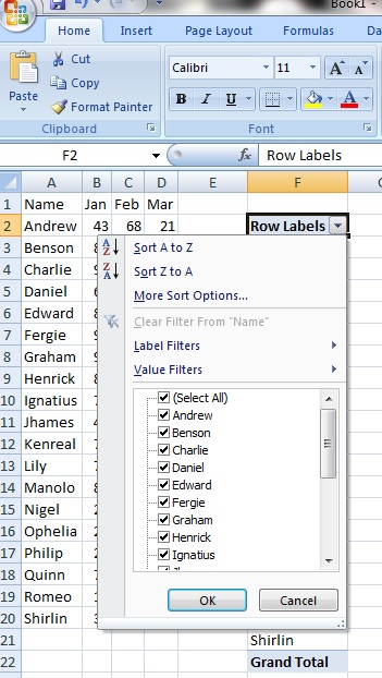
By clicking on the dropdown arrow you can actually manipulate the list by sorting it in ascending order using ‘Sort A to Z’ or descending order using ‘Sort Z to A’ or even take out some names by unchecking the arrows next to each name.
Step 7:
Now, click and drag all the other field names from ‘Jan’ to ‘Mar’ into the ‘Values’ box.

Done! Now you have a table with the grand total of all the sales made for each month from January to March.
Tip 1:
You can change how the data is processed. Say, you want to count the total number of instances instead of adding them all up.
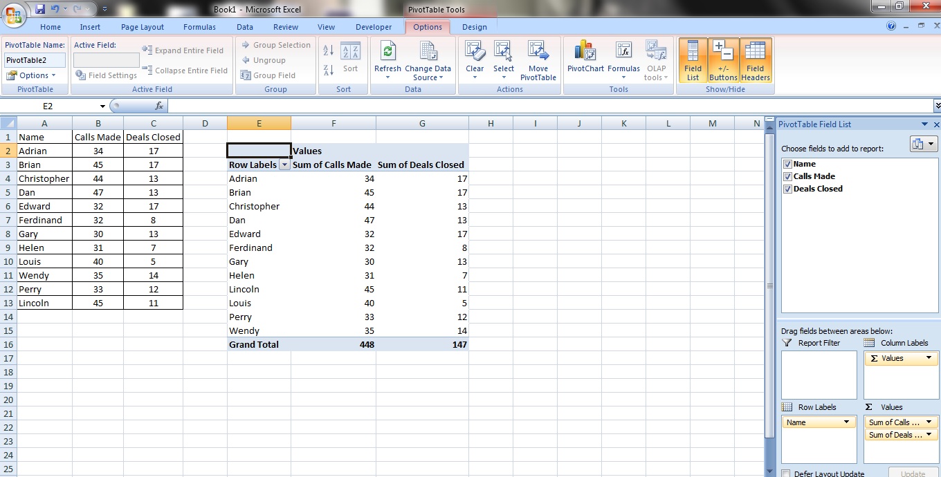
Here we have a pivot table displaying the calls and deals closed for several colleagues:
Step 1:
To change the way the data is displayed, go to the menu at the bottom right.
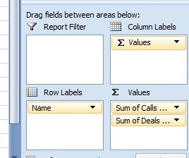
Step 2:
By left clicking on any of the fields under ‘Values’, you will see this menu.
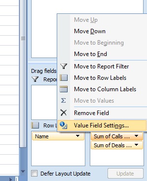
Select ‘Value Field Settings…’.
Now, a whole list of options will appear for you to select on whether you want your data summed, counted or even averaged!
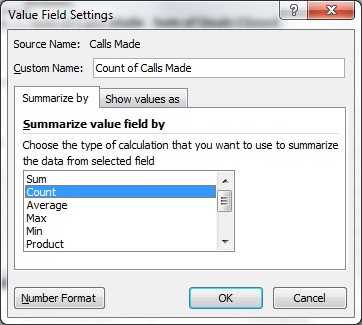
Step 3:
Let’s just select ‘Count’ for illustration.
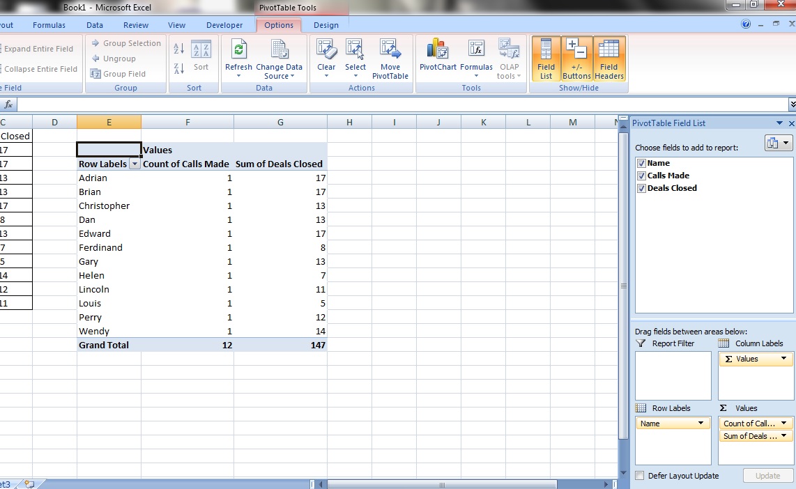
Notice that the data for calls made are no longer summed? What we have done is COUNTED the instances where numbers appear for each of the colleagues – that means that we have counted the number of times any calls have been made at all.
Tip 2:
Did you know that pivot tables add up values corresponding to repeated names?
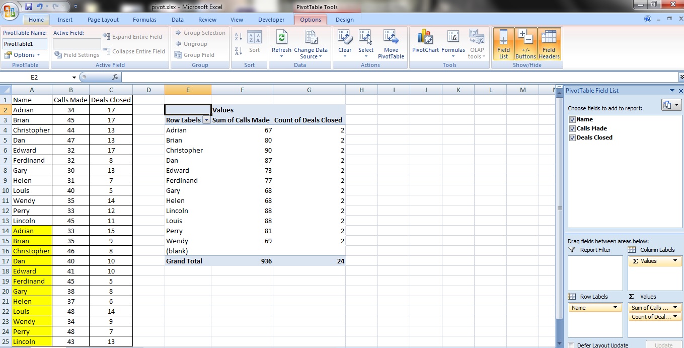
Consider this database. Notice that the names in yellow are repeats of the names above? Name for name.
Applying a normal pivot table’s procedures to the data, the pivot table displays the combined values added up, WITH NO REPEATED NAMES!
This means that the pivot table knows when a name is repeated and instead of just reproducing the data, adds it to a matching existing name. Saves you tonnes of time!

Leave a comment