Excel’s Most Important Function.

Functions 9: VLOOKUP

Time to learn: 25 minutes

You will find this perhaps the most powerful function within the Excel framework. Why? Because one of the most tedious tasks in data management is keeping track of it all.

During the age of the dinosaurs, if you had 10 items to keep track of, that would be no problem, but due to the scale at which the world is now used to, a relatively small piece of data would be thousands, if not hundreds of thousands of items long.

VLOOKUP effectively and efficiently cross-checks and compares lists in seconds.

So, let’s get our hands around this and choke it.

VLOOKUP

The VLOOKUP function is essentially a function that COMPARES LISTS. So, it would look at one list of items and tell you if another list you have contains the same items.

If you had a list of all the items in your store and a client asked you if you could supply him a list of items, you could check if your store could fulfil that order in maybe, 5 seconds. Instead of going through each and every item to cross-check, VLOOKUP does it for you.

Here is our inventory list in column A and our price list in column B. Apparently everything a warrior poet needs.

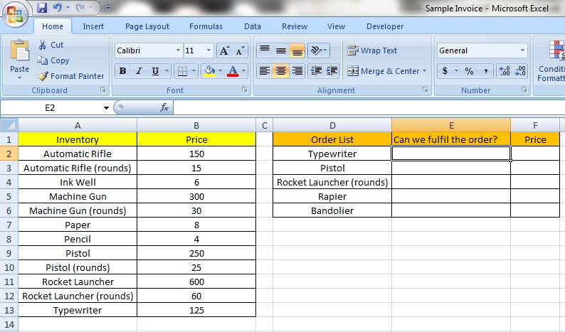
In column D is our client’s order list and in column E, blank cells for us to put a formula in to determine whether we have the item in stock and column F, which we will put another VLOOKUP formula into to determine the price of the item if we have it.

Here’s an example:

=VLOOKUP(D2,A:B,1,FALSE)

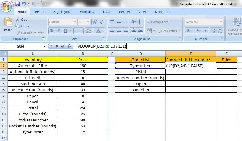
The structure of the VLOOKUP function starts with the ‘=’, as all formulas do. Then the VLOOKUP function comes next and then the contents framed in ‘(‘ and ‘)’.

How about the contents?

D2 refers to the first item that you want to confirm is in the inventory list – in this instance, it is a Typewriter (which I am sure you may not have used or seen before). The cell below this would refer to D3, the Pistol, as it is the 2^nd item, D4 would refer to the 3^rd item, the Rocket Launcher (rounds) and so on.

Let’s call the next part, consisting of columns A and B, the Comparison Table. A:B, as you have probably noticed, is a column label reference consisting of 2 columns.  This means that the whole of column A and B have been selected.  So, our Comparison Table consists of column A, which is the list of the store’s inventory and column B, which is the price of each item

*A point to note – this is crucial! The items in D2, for that matter, in column D, must be the items that you want to compare against in the 1^st column of the Comparison Table, in this case, column A as it is the 1^st column.  The contents of D2 must be of the same type as those in the 1^st column of your Comparison Table – in this case, the names of items.

How about the 1? This is a column reference and it means that we are checking the contents of D2 against the contents in the 1^st column of A:B.  That’s because all we want to do is confirm whether the item in D2 is in the inventory list of column A.

What if we wanted to know just the price? As you have guessed, we change the 1 to 2, meaning that we want to compare the contents of D2 with the items in column A and to get back the contents of column B, the 2^nd column in our Comparison Table, hence the 2, which would be the price of the item.

This just gives us the price of the item, though and not its name. So, if we wanted to check whether the item in D2 is within column A and to ALSO know the price of the item from column B, we would have to have 2 VLOOKUP formulas.

You must type either TRUE or FALSE in the final part of the structure.

FALSE means that you want VLOOKUP to match the contents of D2 EXACTLY against the contents of A:A, letter for letter, number for number, word for word.

Typing TRUE means that you want an approximate match, meaning that if the contents of D2 are close to that of A:A, then the contents of A:A appear. Though this is useful for certain purposes, it is usually not what we are looking for.

Here’s what I mean:

=VLOOKUP(D5,A:B,1,TRUE)

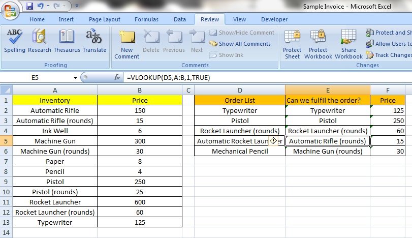
Now, we know that we don’t sell Automatic Rocket Launchers or Mechanical Pencils, but Excel has returned values that are closest to them, Automatic Rifle (rounds) being the closest to Automatic Rocket Launchers and Machine Gun (rounds) being the closest to Mechanical Pencil.

Now, let’s copy the formula to the cells below.

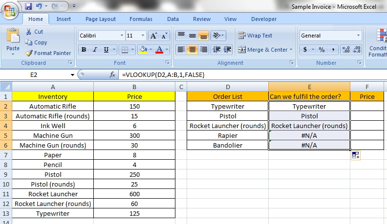
If we have the items, the formula gives us the name of the item, meaning that it is within the inventory list in column A.

We see that we can only supply the 1^st 3 items and that we do not have the Rapier and the Bandolier.  We know this as the cells with the formula beside the Rapier and Bandolier have retuned us #N/A. Oh, well.

Let’s also get the prices of the items that we can supply to our client. Here’s the formula:

=VLOOKUP(D2,A:B,2,FALSE)

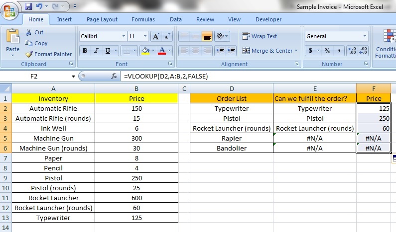
As in the first VLOOKUP formula, when we copy the cells downwards, we see that the 1^st 3 items have their prices indicated, but for the Rapier and Bandolier only the #N/A is displayed.  This is what we are expecting – no item, no price.

Now, what if you wanted to remove the #N/As so that it looks nice? Well, we will get to that in another lesson.