Be THE MAN in your company with an interactive database!

Sample 2: Interactive Database

We all work with data – tonnes of it.  Ever wanted to find all the information you need, with just 1 click of the mouse?

Let’s build an INTERACTIVE DATABASE.

Time to learn: 30 minutes

Functions you will need:

1. Data Validation
2. Vlookup
3. Conditional Formatting

Step 1:

Let’s start with some data.

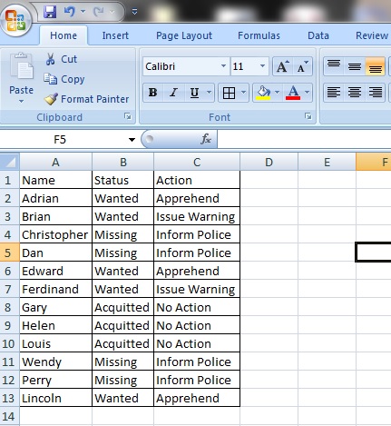
Here is a list of suspects in a database.  All of them have a name and a ‘Status’, whether they are ‘Wanted’, ‘Acquitted’ or ‘Missing’.  They also have a column next to their ‘Status’, indicating the ‘Action’ to be taken if they are seen – to ‘Apprehend’, ‘Issue Warning’ or just to ‘Inform Police’.

Step 2:

Let’s create a dropdown list of all the suspects in our list.

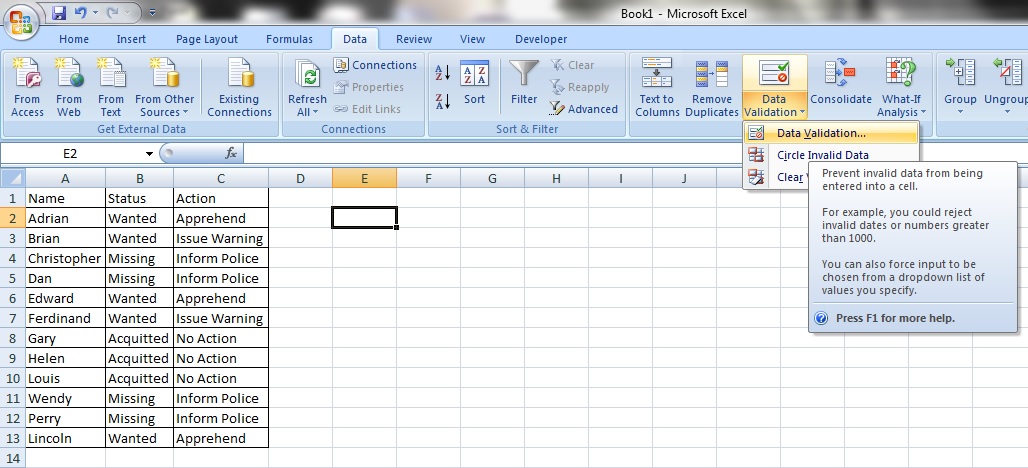
Go to ‘Data’ tab and select ‘Data Validation’.  Select ‘Data Validation’ again.

Step 3:

An option box will appear with the title ‘ Data Validation’.

Under the field ‘Allow:’, select the option ‘List’ and click ‘OK’.

Step 4:

In the field named ‘Source’, click and drag on the list of cells with the names of all the suspects, from cells A2 to A13.

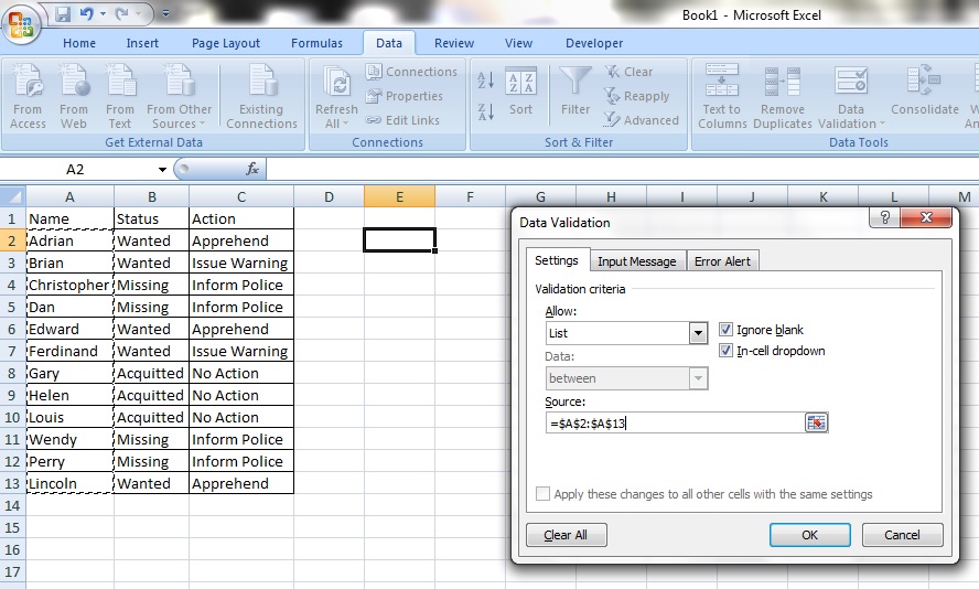
You will see that the list of names now has a dotted line bordering it and the ‘Source’ field now has the reference ‘=$A$2:$A$13’.  Click ‘OK’.

Step 5:

Now you have a dropdown list of all the names of suspects in our database!

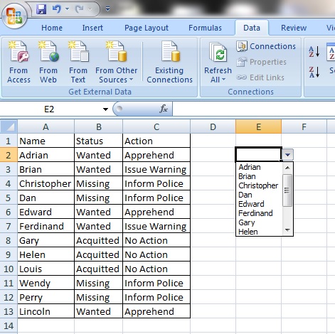
Remember that the dropdown list is presented in EXACTLY the same order as they are in the original list (cells A2 to A13).  You can alter the order of the dropdown list by altering the order in the original list (cells A2 to A13).

Step 6:

Now, type in ‘Name’, ‘Status’ and ‘Action’ as shown.

These will be OUR data titles.

Step 7:

In cell F2, under the title ‘Status’, enter the following VLOOKUP function:

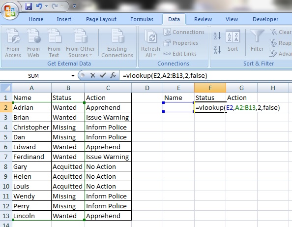
=VLOOKUP(E2,A2:B13,2,FALSE)

E2 refers to the cell that the names of the suspects will appear in from our dropdown list.

A2:B13 is the complete cell reference of all the suspects’ ‘Name’ and ’Status’.

2 refers to the option that we have specified –that we want the information in the 2^nd column to the right of the suspect’s name, counting the suspect’s name as well (meaning ‘Name’ being the 1^st column and ‘Status’ being the 2^nd column), to appear in the cell we have currently selected – F2.

Step 8:

Do the same in the cell under ‘Action’ –cell G2:

=VLOOKUP(E2,A2:C13,3,FALSE)

E2 refers to the cell that the names of the suspects will appear in from our dropdown list.

A2:C13 is the complete cell reference of all the suspects’ ‘Name’, ’Status’ and ’Action’ .

3 refers to the option that we have specified –that we want the information in the 3^rd column to the right of the suspect’s name, counting the suspect’s name as well (meaning ‘Name’ being the 1^st column, ‘Status’ being the 2^nd column and ‘Action’ being the 3^rd column), to appear in the cell we have currently selected – G2.

Step 9:

Now, when we select any name from the dropdown list in E2, their ‘Status’ and ‘Action’ are automatically displayed next to their names!

Step 10:

Let’s make it even more sophisticated!

Click on cell F2.  While still ensuring that the cell F2 is selected, select the ‘Home’ tab and select ‘Conditional Formatting’ then ‘Highlight Cells Rules’ and then ‘Text that Contains…’.

Step 11:

An option box will appear.

In the ‘Format cells that contain the text:’ field, enter the text ‘Wanted’.  In the box to the right of that, let’s just select Light Red Fill with Dark Red Text.  Click ‘OK’.

Step 12:

Follow step 10 again and this time, in the ‘Format cells that contain the text:’ field, enter the text ‘Missing’.  In the box to the right of that, let’s just select Yellow Fill with Dark Yellow Text.  Click ‘OK’.

Step 13:

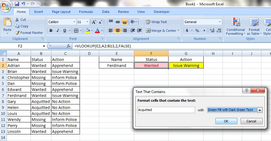
Follow step 10 again and this time, in the ‘Format cells that contain the text:’ field, enter the text ‘Acquitted’.  In the box to the right of that, let’s just select Green Fill with Dark Green Text.  Click ‘OK’.

Step 14:

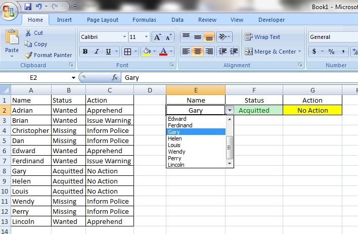
NOW, when you select the name ‘Gary’, notice that the ‘Status’ of ‘Acquitted’ is now coloured in green?  You have just formatted the cell F2 to respond to the different ‘Status’ types by changing colour!  Great job!

Notice the change now when you select the name ‘Wendy’.  Cool, right?

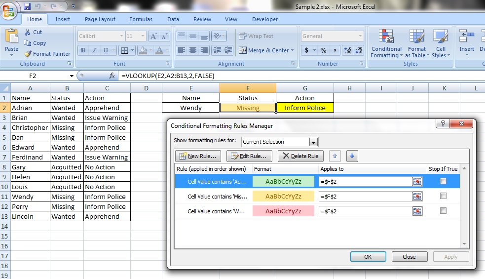
Tip:

You can see how many formats you have programmed into the cell by selecting the cell and then by selecting the ‘Home’ tab, ‘Conditional Formatting’ and then ‘Manage Rules’.

Notice that we have programmed 3 rules into cell F2 that change the colour of the cell depending on whether the text in it is ‘Wanted’, ‘Missing’ or ‘Acquitted’.

Excellent work!