Make your spreadsheet look like a MILLION BUCKS!

Aesthetics 1: Data Validation

Time to learn: 10 minutes

Want to make your spreadsheet look ultra-professional and have people asking you for weeks how you did it?

You are going to love this. Data Validation is a sweet term for dropdown lists, which we are going to be creating today!

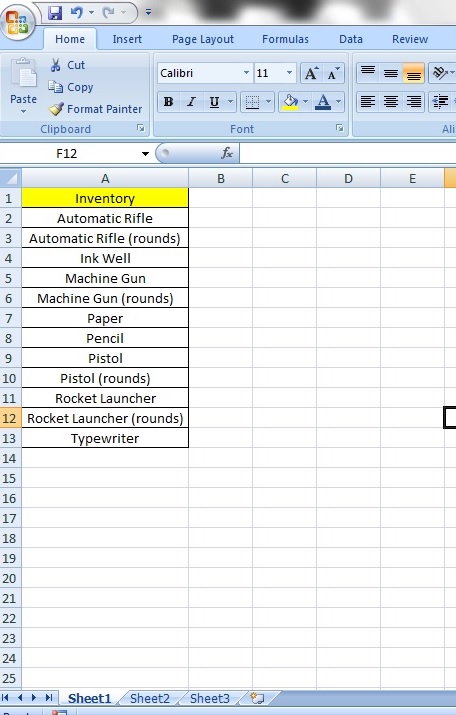
So, let’s start with some data to create a list of items for sale:

Once again, we will use the items we are selling to equip aspiring warrior-poets.

Now, here are the steps for creating a drop-down list of all these items.

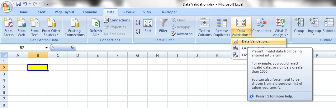
Step 1:

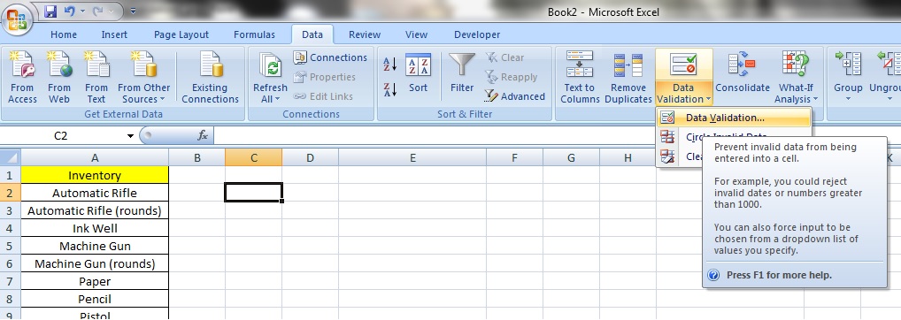
Go to the ‘Data’ tab and select ‘Data Validation’ – a drop down arrow will show 3 options – select ‘Data Validation’ once again.

Step 2:

Once you have selected the ‘Data Validation’ option, an option box will appear.  In the option box for ‘Data Validation’, under ‘Allow’, select ‘List’.

Step 3:

Upon selecting the ‘List’ option the option box will expand and you will see the ‘Source’ box – this is essentially the contents you want in the dropdown box. Select the items you want.  In this case, all our items for sale, which are from cells A2 to A13.

Notice that the title ‘Inventory’ is NOT selected.

Now, press the ‘OK’ button.

Step 4:

Done!

Now you will see a dropdown box and upon clicking on the dropdown arrow, the list of items has appeared.

Easy!

Tip:

By now you would have noticed that the data validation list can only appear on the same sheet as the referenced list.

What if you wanted to place the reference list in a different sheet from the data validation list?  Possible!

Step 1:

Here we have our data list.  Notice that it exists on Sheet 1.  We will now make a data validation list on Sheet 2.

Step 2: 

Select the cell range that you want to appear in our data validation list.  I’ve selected just the names of the items from cell A2 to A13.  Perform a right click and select ‘Name a Range…’ from the menu options.

Step 3:

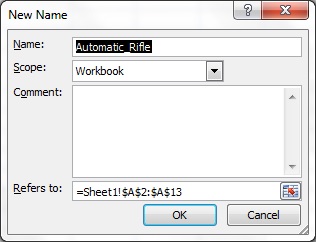
You will see this option box appear.  In the field ‘Refers to:’, notice that the cell reference is exactly the one we selected previously?

Leave the field ‘Scope’ as it is.  Having ‘Workbook’ in the ‘Scope’ field means that the list will apply wherever in the workbook that we refer to it.

Step 4:

In the ‘Name’ field, type the text ‘List’.  This means we are naming our list of items ‘List’.

Step 5:

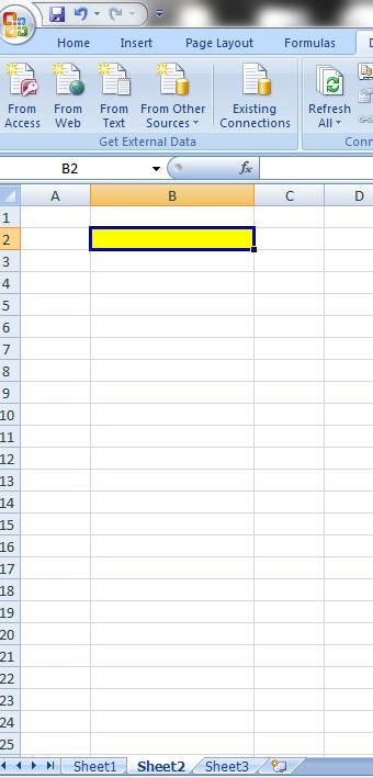
Now, let’s move to Sheet 2.  Notice that I have coloured one of the cells yellow – that’s where we will place our data validation list.

Step 6:

Go to the ‘Data’ tab and then to the ‘Data Tools’ category and select ‘Data Validation’.  Select ‘Data Validation’ again.

 

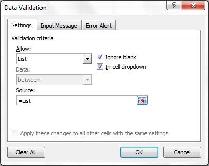
Step 7:

This option box will appear.  Under the ‘Allow’ field, select ‘List’.

Step 8:

Now, in the ‘Source’ field, type in =List.  Recall that we named our reference list as ‘List’.  We are referring to it here!  Now, click ‘OK’.

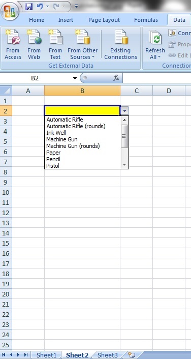
Step 9:

There you have it!  A data validation list that appears in a separate list from the reference list.  This makes for a much neater appearance and a more professional feel to your spreadsheet!