excelpunks. Training – Consultancy – Solutions.

Function: IF, AND & OR

Want to know how to make your spreadsheet look like it’s a thinking being?  Looking for a way to make your data talk back to you?

The most interesting aspect about Excel is the ability to execute logical equations or FUNCTIONS.

IF

One of my favourite functions is the IF function. Remember that this is a formula and as such, whenever you type it into a cell, you have to begin with a ‘=’ sign.

The structure of the IF function has 3 parts and looks like this:

=if(1. a logical or mathematical expression; usually referring to another cell, like if cell A1 is equal to 3 or if cell A1 is equal to cell B1, 2.then what you would like this cell to say or do if the expression indicated in 1. is true, 3. Lastly, what you would like this cell to say or do if the expression in 1. is false)

Here’s an example:

=if(A1=3,1,0)

 

What I have done is create an IF function that checks if cell A1 is equal to 3. If it is equal to 3, the cell the formula is in then gives you a value of 1.  If cell A1 is any other value besides 3, the cell then gives you a value of 0.  So, what right?

Like so many things in Excel, the IF function is so, so much more!

Here’s another example:

=IF(A1=3,”I do not want a 3!”,”Not a 3 is fine.”)

Notice that the text in the IF function is framed by “ ”. All text in any function – if you want it to behave like text, must be framed by “ ”.  What we have done is create a function that checks whether cell A1 is equal to 3.  If cell A1 is equal to 3, the cell then gives you the text, “I do not want a 3!”.

If cell A1 is any other value except 3, the cell then gives you the text, ”Not a 3 is fine.”

This makes for wonderfully interactive formulas that not only do the work, but add personality!

Again, so what? Really?

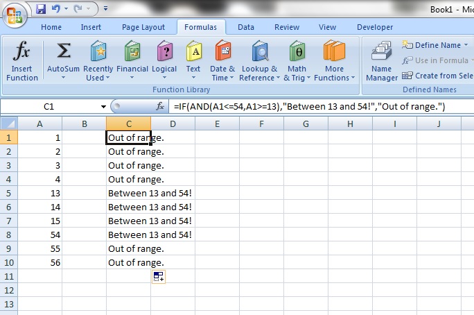
Here’s another one. Let’s say you have 1,000 random numbers ranging from 0 to 9999 and you wanted to know which ones were between 13 and 54.

Here’s how we’d do it:

=IF(AND(A1<=54,A1>=13),”Between 13 and 54!”,”Out of range.”)

Whoa, what the hell was that? The IF function allows a combination with 2 other types of functions, AND and OR.  We’ll talk about that in a moment.

So the formula above says that if cell A1 is less than or equal 54, indicated by the <= AND if cell A1 is ALSO more than or equal to 13, indicated by the >=, then the cell tells you, “Between 13 and 54!”. If cell A1 is outside of this magical 13 -54 range, the cell then says, “Out of range.”

The best part is that by placing your mouse pointer at the LOWER RIGHT corner of a cell, then holding the left-button, you can move the mouse pointer downwards, thereby COPYING the formula onto the cells below. Dragging upwards copies the cell contents upwards too.  You will notice that in the cell along the same row as A9, the formula does not mention cell A1 anymore, but A9.

Neat, huh?

AND

The AND function is used in combination with the IF function to add more logical expressions to the first one.

So, the example:

=IF(AND(A1<=54,A1>=13), “Between 13 and 54!”,”Out of range.”)

Means that BOTH the conditions A1<=54 and A1>=13 MUST be fulfilled before the text “Between 13 and 54!” appears. Otherwise, “Out of range.” appears instead.

OR

The OR function is similar to the AND function, but as you probably guess, you sly fox you, when used in combination with the IF function, assesses whether EITHER of the logical expressions is fulfilled before returning the values if the expressions are true.

Here’s an example:

=IF(OR(A2=1,B2=1),”Team 1 in Season 1 or 2″,”Team 1 absent”)

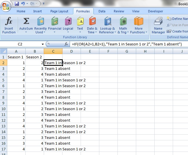
Let’s take the columns A and B as a team roster for Seasons 1 and 2. The expression using IF and OR above checks whether Team 1 is in EITHER Season 1 or 2, giving you the text, “Team 1 in Season 1 or 2″.  If Team 1 is absent from both seasons, the text, “Team 1 absent” presents itself.

Now, note the difference if we had used IF and AND instead:

=IF(AND(A2=1,B2=1),”Team 1 in Season 1 or 2″,”Team 1 absent”)

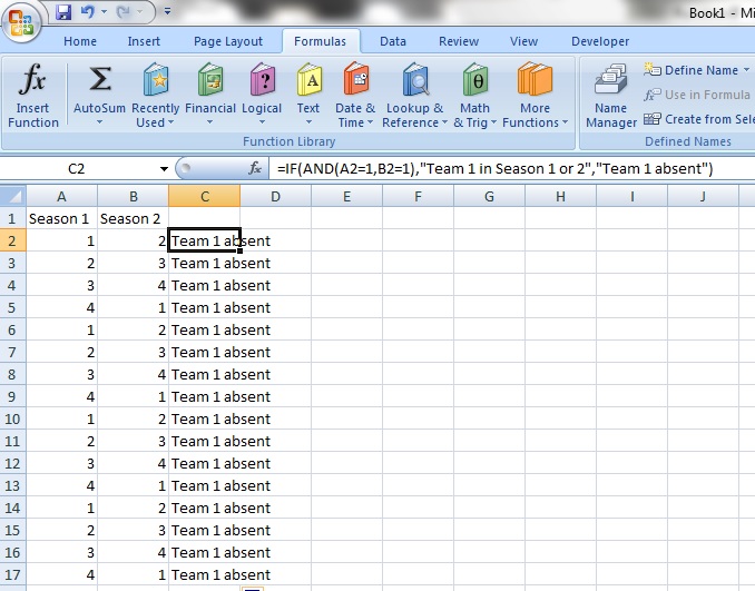
Remember that the IF and AND function when used together, checks if BOTH expressions are true before returning the text, “Team 1 in Season 1 or 2″. Since Team 1 is only in either Season 1 or 2 but never both at the same time, “Team 1 absent” is returned.  This happens because, yes, BOTH conditions, that Team 1 would be in Season 1 and 2 at the same time, were not met.

I hope this gives you a good illustration of how the AND and OR functions work and their differences. Did I mention that you can use IF, AND and OR at the same time?  Okay, okay, another time.

Here’s something extra:

Let’s say you have 9 teams, named 1 through 9 and you want to group teams 1 to 3 into a separate team, called Team Badger, teams 4 to 6 into another team, called Team Skunk and teams 5 to 9 into a final team called Team Dead. How would we do that? Here’s how:

=IF(OR(A2=1,A2=2,A2=3),”Team Badger”,IF(OR(A2=4,A2=5,A2=6),”Team Skunk”,IF(OR(A2=7,A2=8,A2=9),”Team Dead”,”Not a Team”)))

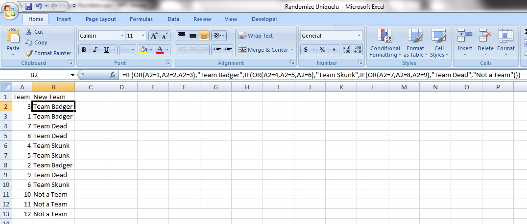
So, not only are we able to identify the teams to be grouped into new teams when they aren’t in order, we are also able to tell when there are values not in our desired line up.

Here’s something extra:

Often, you may want to make use of the logical aspects of the IF function to do interesting things.

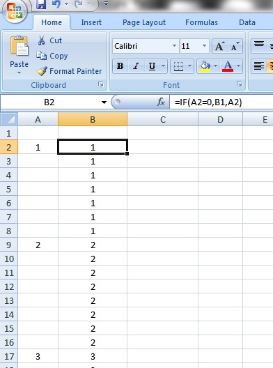
When working with large amounts of data, you may encounter a situation like this where you need to copy numbers multiple times in order to fill up gaps. It is a REAL PAIN.

So, using the IF function, we would be able to fix that. Here’s how:

=IF(A2=0,B1,A2)

Voodoo!!!